Lecture 4: Introduction to Reinforcement Learning

Lecture Slides & Videos

• Lecture 4: Introduction to Reinforcement Learning

• CS 285: Lecture 4, Part 1

• CS 285: Lecture 4, Part 2

• CS 285: Lecture 4, Part 3

• CS 285: Lecture 4, Part 4

• CS 285: Lecture 4, Part 5

• CS 285: Lecture 4, Part 6

Definitions

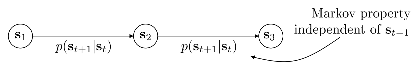
Markov chain

$$ \mathcal{M} = {\mathcal{S}, \mathcal{T}} $$

• $\mathcal{S}$ — state space

  • state $\mathcal{s} \in \mathcal{S}$ ( discrete or continuous )

• $\mathcal{T}$ — transition operator

  • $p(s_{t+1}|s_t)$

  • let $\mu_{t,i}=p(s_{t}=i)$, then $\vec{\mu}_t$ is a vector of probabilities

    let $\mathcal{T}_{i,j}=p(s_{t+1}=i|s_t=j)$, then $\vec{\mu}_{t+1}=\mathcal{T}\vec{\mu}_t$

  

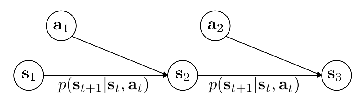
Markov decision process

$$ \mathcal{M} = {\mathcal{S, A, T, r}} $$

• $\mathcal{S}$ — state space
  • state $\mathcal{s} \in \mathcal{S}$ ( discrete or continuous )
• $\mathcal{A}$ — action space
  • state $\mathcal{a} \in \mathcal{A}$ ( discrete or continuous )
• $\mathcal{T}$ — transition operator ( now a tensor )
  • let $\mu_{t,i}=p(s_{t}=i)$
  • let $\xi_{t,k}=p(a_t=k)$
  • let $\begin{aligned} \mathcal{T}_{i,j,k}=p(s_{t+1}=i|s_t=j,a_t=k) \end{aligned}$
  • then $\begin{aligned} \mu_{t+1,i}=\sum_{j,k}\mathcal{T}_{i,j,k}\mu_{t,j}\xi_{t,k} \end{aligned}$
• $\mathcal{r}$ — reward function
  • $r:\mathcal{S}\times\mathcal{A}\to\mathbb{R}$

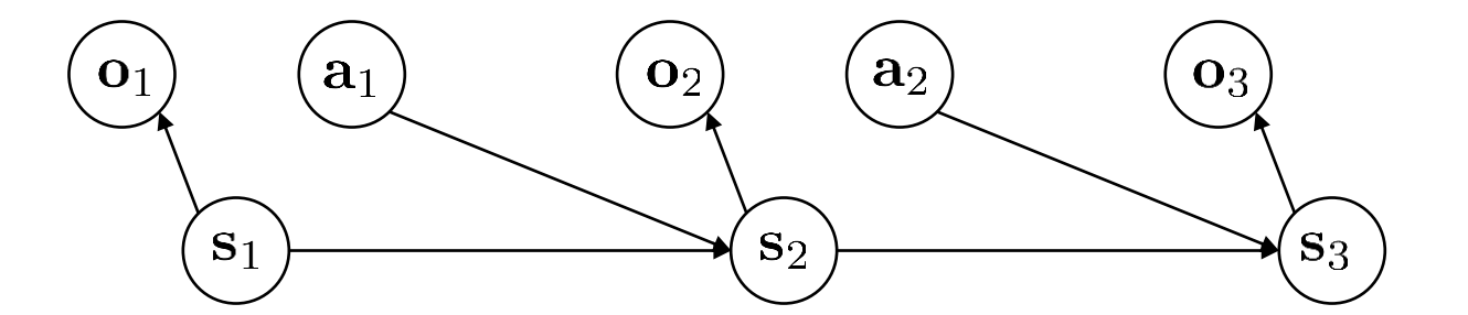
Partially observed Markov decision process

$$ \mathcal{M} = {\mathcal{S, A, O,T, E, r}} $$

• $\mathcal{O}$ — observation space
  • observations $\mathcal{o} \in \mathcal{O}$ ( discrete or continuous )
• $\mathcal{E}$ — emission probability
  • $p(o_t | s_t)$

The goal of reinforcement learning

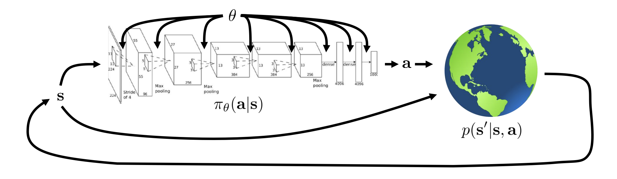
$$ p_\theta(\mathbf{s}_1,\mathbf{a}_1,\ldots,\mathbf{s}_T,\mathbf{a}_T)=p(\mathbf{s}_1)\prod_{t=1}^T\pi_\theta(\mathbf{a}_t|\mathbf{s}_t)p(\mathbf{s}_{t+1}|\mathbf{s}_t,\mathbf{a}_t) $$

where $\tau = \mathbf{s}_1,\mathbf{a}_1,\ldots,\mathbf{s}_T,\mathbf{a}_T$ is called trajectory, a sequence of states and actions.

Therefore, we can define an objective for reinforcement learning: to find the parameters $\theta$ that define our policy so as to maximize the expected value of the sum of the rewards over the trajectory.

$$ \begin{aligned}\theta^\star=\arg\max_\theta E_{\tau\thicksim p_\theta(\tau)}\left[\sum_tr(\mathbf{s}_t,\mathbf{a}_t)\right]\end{aligned} $$

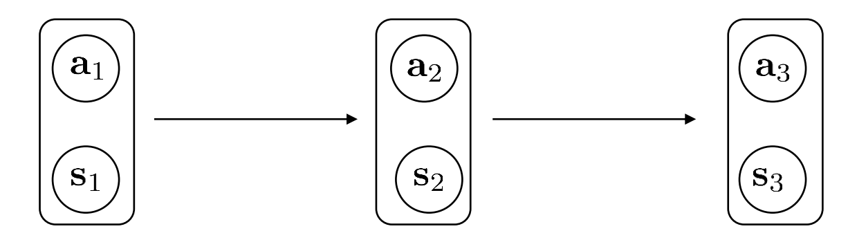
Finite horizon case: state-action marginal

We can group the state and action together into a kind of augmented state, which actually from a Markov chain.

$$ p((\mathbf{s}_{t+1},\mathbf{a}_{t+1})|(\mathbf{s}_t,\mathbf{a}_t))=p(\mathbf{s}_{t+1}|\mathbf{s}_t,\mathbf{a}_t)\pi_\theta(\mathbf{a}_{t+1}|\mathbf{s}_{t+1}) $$

Therefore, we can define the object in a slightly different way

$$ \theta^\star=\arg\max_\theta\sum_{t=1}^TE_{(\mathbf{s}_t,\mathbf{a}_t)\sim p_\theta(\mathbf{s}_t,\mathbf{a}_t)}[r(\mathbf{s}_t,\mathbf{a}_t)] $$

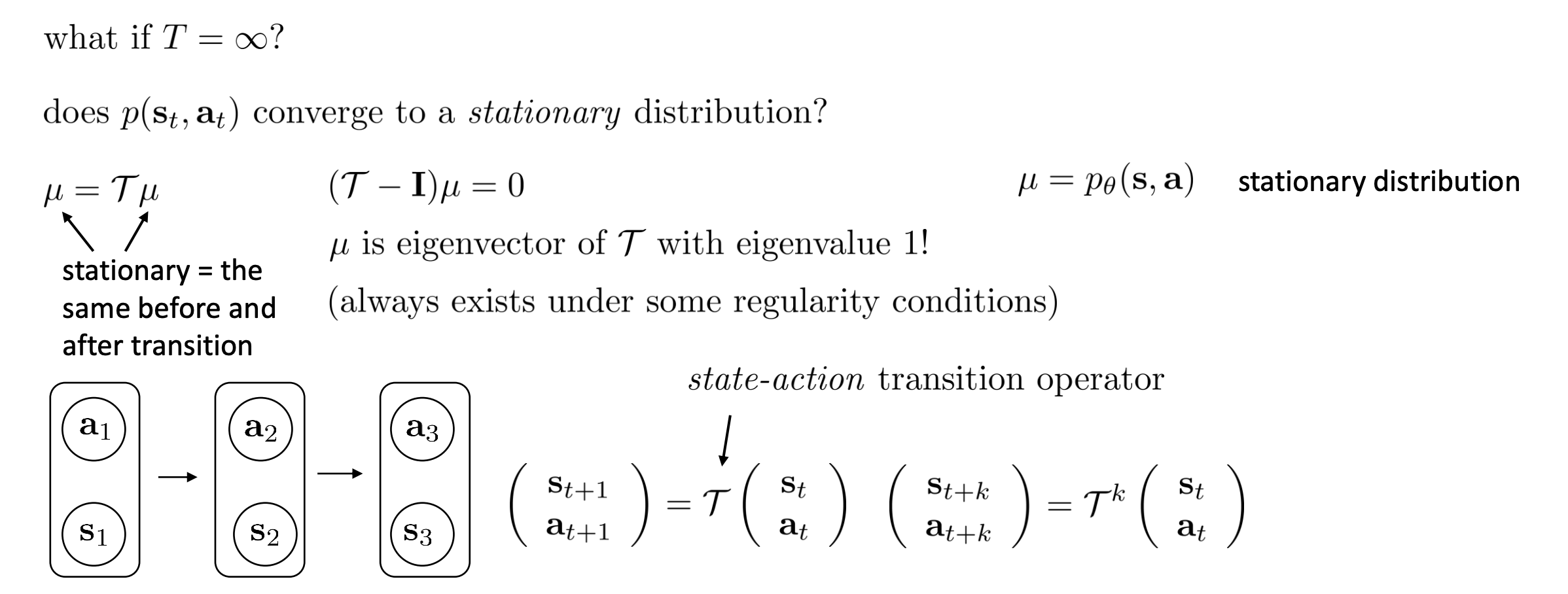
Infinite horizon case: stationary distribution

Expectations and stochastic systems

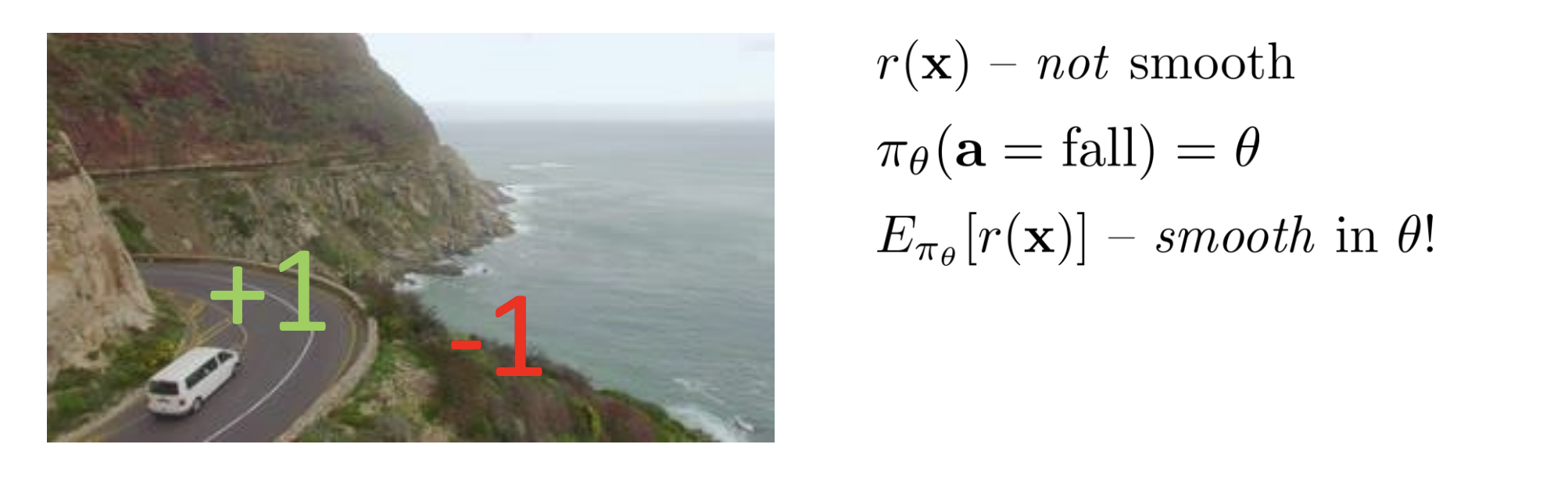
Reinforcement learning is really about optimizing expectations.

Although we talk about reinforcement learning in terms of choosing actions that lead to high rewards, we’re always really concerned about the expected values of rewards.

The interesting thing about the expected values is that the expected values can be continuous in the parameters of the corresponding distributions even when the function that we’re talking the expectation of is itself highly discontinuous, which is the reason why reinforcement learning algorithms can use smooth optimization methods like gradient descent to optimize objective that are seemingly non-differentiable, like binary rewards for winning or losing a game.

Algorithm

The anatomy of a reinforcement learning algorithm

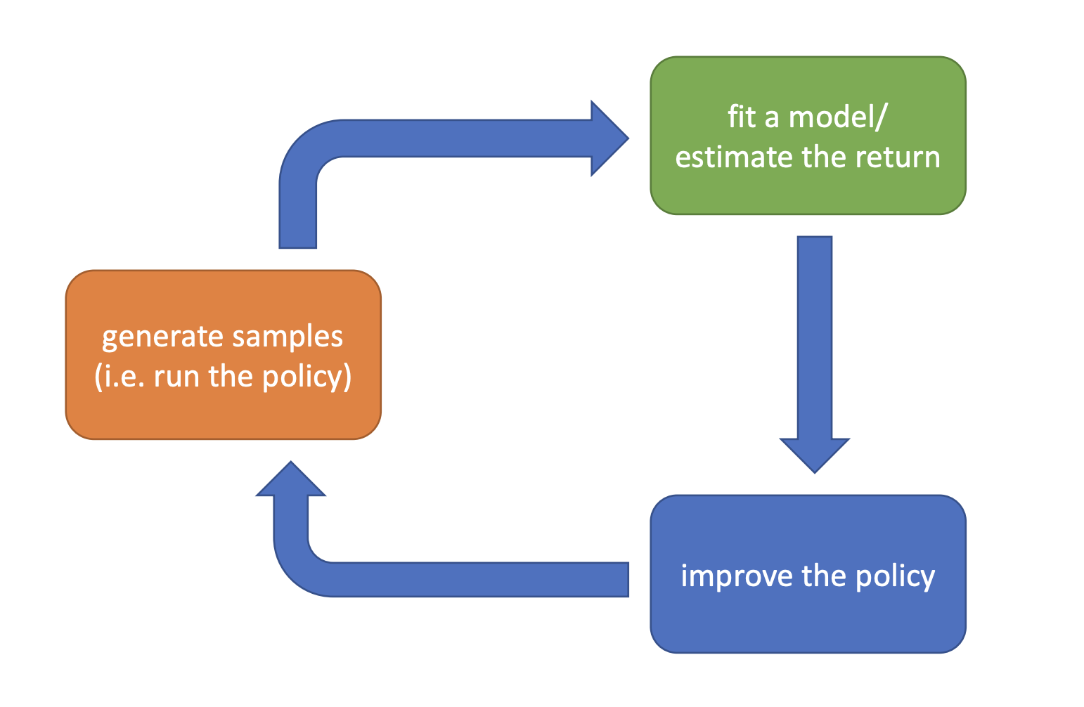
Which parts are expensive?

• generate samples
  • If we use a real robot real world, it will be rather expensive.
  • If we use a simulator, the cost might be trivial.
• fit a model/estimate the return
  • If we just sum up the rewards we obtained, this might be rather cheap.
  • If we are learning an entire model by training a whole of neural net, this might require a big supervised learning run in the inner loop of the RL algorithm.
• improve the policy
  • If we are just taking one gradient step, this might be rather cheap.
  • If we have a backprop through the model, this might be rather expensive.

Value Functions

How do we deal with all these expectations?

As mentioned above, the reinforcement learning objective can be defined as an expectation

$$ E_{\tau\sim p_\theta(\tau)}\left[\sum_{t=1}^Tr(\mathbf{s}_t,\mathbf{a}_t)\right] $$

We can actually write it out recursively

$$ E_{\mathbf{s}_{1}\sim p(\mathbf{s}_{1})}\left[E_{\mathbf{a}_{1}\sim\pi(\mathbf{a}_{1}|\mathbf{s}_{1})}\left[r(\mathbf{s}_{1},\mathbf{a}_{1})+E_{\mathbf{s}_{2}\sim p(\mathbf{s}_{2}|\mathbf{s}_{1},\mathbf{a}_{1})}\left[E_{\mathbf{a}_{2}\sim\pi(\mathbf{a}_{2}|\mathbf{s}_{2})}\left[r(\mathbf{s}_{2},\mathbf{a}_{2})+…|\mathbf{s}_{2}\right]|\mathbf{s}_{1},\mathbf{a}_{1}\right]|\mathbf{s}_{1}\right]\right] $$

What if we have some functions that tells us $Q(\mathbf{s}_1,\mathbf{a}_1)$, where

$$ Q(\mathbf{s}_1,\mathbf{a}_1)=r(\mathbf{s}_1,\mathbf{a}_1)+E_{\mathbf{s}_2\sim p(\mathbf{s}_2|\mathbf{s}_1,\mathbf{a}_1)}\left[E_{\mathbf{a}_2\sim\pi(\mathbf{a}_2|\mathbf{s}_2)}\left[r(\mathbf{s}_2,\mathbf{a}_2)+…|\mathbf{s}_2\right]|\mathbf{s}_1,\mathbf{a}_1\right] $$

• Q-function: total reward from taking $\mathbf{a}_t$ in $\mathbf{s}_t$

$$ Q^\pi(\mathbf{s}_t,\mathbf{a}_t)=\sum_{t^{\prime}=t}^TE_{\pi_\theta}\left[r(\mathbf{s}_{t^{\prime}},\mathbf{a}_{t^{\prime}})|\mathbf{s}_t,\mathbf{a}_t\right] $$

• Value function: total reward from $\mathbf{s}_t$

$$ V^{\pi}(\mathbf{s}_{t})=\sum_{t^{\prime}=t}^{T}E_{\pi_{\theta}}[r(\mathbf{s}_{t^{\prime}},\mathbf{a}_{t^{\prime}})|\mathbf{s}_{t}] = E_{\mathbf{a}_{t}\sim\pi(\mathbf{a}_{t}|\mathbf{s}_{t})}[Q^{\pi}(\mathbf{s}_{t},\mathbf{a}_{t})] $$

Therefore, the reinforcement learning objective can be modified as

$$ E_{\mathbf{s}_1\sim p(\mathbf{s}_1)}[V^\pi(\mathbf{s}_1)] $$

Using Q-functions and value functions

Idea 1: if we have policy $\pi$, and we know $Q^{\pi}(\mathbf{s},\mathbf{a})$, then we can improve $\pi$:

• set $\pi^{\prime}(\mathbf{a} | \mathbf{s}) = 1$ if $\mathbf{a} = \arg\max_\mathbf{a}Q^\pi(\mathbf{s},\mathbf{a})$
  • this policy is at least as good as $\pi$ and probably better
  • it doesn’t matter what $\pi$ is

Idea 2: compute gradient to increase probability of good actions $\mathbf{a}$

• if $Q^\pi(\mathbf{s},\mathbf{a}) \gt V^\pi(\mathbf{s})$, then $\mathbf{a}$ is better than average
  • modify $\pi(\mathbf{a} | \mathbf{s})$ to increase probability of $\mathbf{a}$ if $Q^\pi(\mathbf{s},\mathbf{a}) \gt V^\pi(\mathbf{s})$

Types of Algorithms

As we have mentioned above, we are going to optimize the RL objective

$$ \begin{aligned}\theta^\star=\arg\max_\theta E_{\tau\thicksim p_\theta(\tau)}\left[\sum_tr(\mathbf{s}_t,\mathbf{a}_t)\right]\end{aligned} $$

• Policy gradients: directly differentiate the above objective $\Rightarrow$ gradient descend procedure
• Value-based: estimate value function or Q-function of the optimal policy ( no explicit policy )
  • value function or Q-function themselves are typically represented by a neural network
• Actor-critic: estimate value function or Q-function of the current policy, use it to improve policy
• Model-based RL: estimate the transition model, and then…
  • Use it for planning ( no explicit policy )
  • Use it to improve a policy
  • Something else

Model-based RL algorithms

• Learn $p(\mathbf{s}_{t+1}|\mathbf{s}_t,\mathbf{a}_t)$

• This could be a neural net that either outputs a probability distribution over $\mathbf{s}_{t+1}$ or a deterministic model attempting to predict $\mathbf{s}_{t+1}$ directly.

• Just use the model to plan (no policy)

  • Trajectory optimization/optimal control ( primarily in continuous spaces ) – essentially backpropagation to optimize over actions.
  • Discrete planning in discrete action spaces, e.g., Monte Carlo tree search

• Backpropagate gradients into the policy

  • Requires some tricks to make it work

• Use the model to learn a value function

  • Dynamic programming
  • Generate simulated experience for model-free learner

Value function based algorithms

• fit a model/estimate: fit $V(\mathbf{s})$ or $Q(\mathbf{s}, \mathbf{a})$
• improve the policy: set $\pi(\mathbf{s})=\arg\max_\mathbf{a}Q(\mathbf{s},\mathbf{a})$

Direct policy gradient

• fit a model/estimate: $R_{\tau}=\sum_{t}r(\mathbf{s}{t},\mathbf{a}{t})$
• improve the policy: $\theta\leftarrow\theta+\alpha\nabla_\theta E[Q(\mathbf{s}_t,\mathbf{a}_t)]$

Actor-critic

• fit a model/estimate: fit $V(\mathbf{s})$ or $Q(\mathbf{s}, \mathbf{a})$
• improve the policy: $\theta\leftarrow\theta+\alpha\nabla_\theta E[Q(\mathbf{s}_t,\mathbf{a}_t)]$

Tradeoffs Between Algorithms

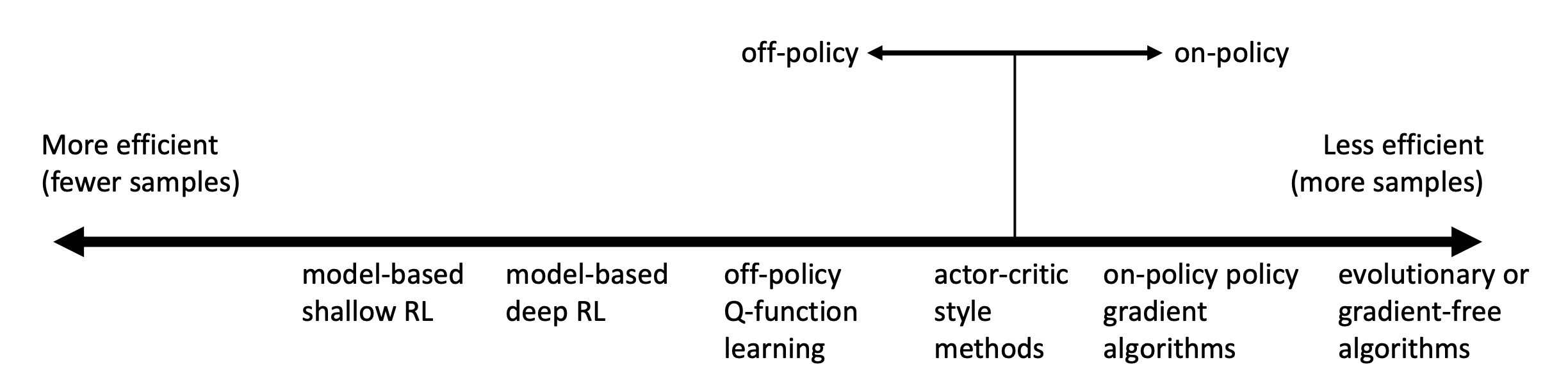
Comparison: sample efficiency

Sample efficiency: how many samples do we need to get a good policy

The most important question is that whether the algorithm is off policy?

• off policy: able to improve the policy without generating new samples from that policy
• on policy: each time the policy is changed, even a little bit, we need to generate new samples

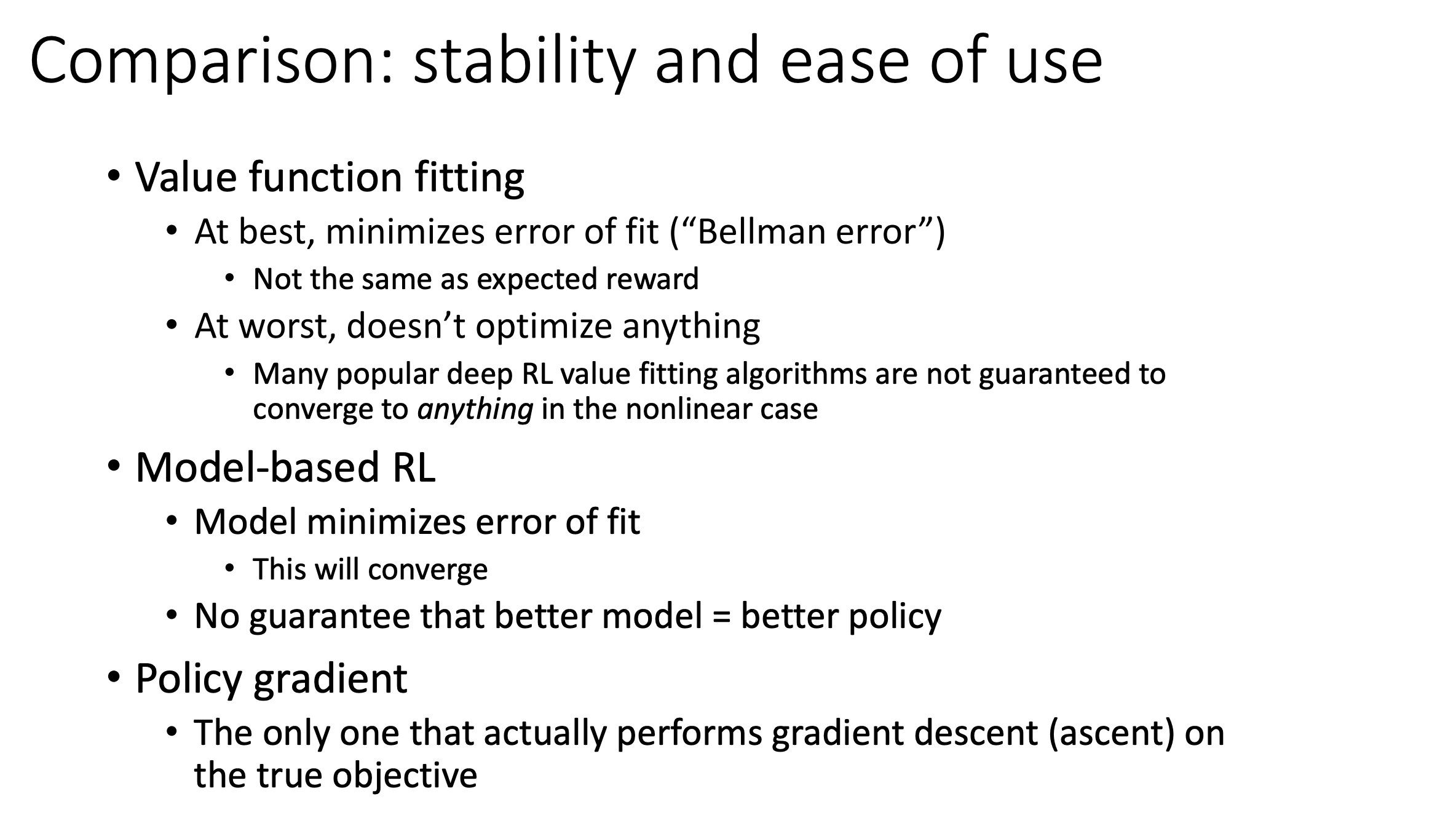
Comparison: stability and ease of use

Supervised learning: almost always gradient descent

Reinforcement learning: often not gradient descent

• Q-learning: fixed point iteration

• Model-based RL: model is not optimized for expected reward

• Policy gradient: is gradient descent, but also often the least efficient!

• Don’t really understand!

  

Comparison: assumptions

• full observability
  • Generally assumed by value function fitting methods
  • Can be mitigated by adding recurrence
• episodic learning
  • Often assumed by pure policy gradient methods
  • Assumed by some model-based RL methods
• continuity or smoothness
  • Assumed by some continuous value function learning methods
  • Often assumed by some model-based RL methods

Examples of Algorithms

• Value function fitting methods
  • Q-learning, DQN
  • Temporal difference learning
  • Fitted value iteration
• Policy gradient methods
  • REINFORCE
  • Natural policy gradient
  • Trust region policy optimization
• Actor-critic algorithms
  • Asynchronous advantage actor-critic (A3C)
  • Soft actor-critic (SAC)
• Model-based RL algorithms
  • Dyna
  • Guided policy search