Lecture 5: Policy Gradient

Lecture Slides & Videos

• Lecture 5: Policy Gradients

• CS 285: Lecture 5, Part 1

• CS 285: Lecture 5, Part 2

• CS 285: Lecture 5, Part 3

• CS 285: Lecture 5, Part 4

• CS 285: Lecture 5, Part 5

• CS 285: Lecture 5, Part 6

Policy Gradient

Evaluating the objective

$$ \theta^\star=\arg\max_\theta E_{\tau\sim p_\theta(\tau)}\left[\sum_tr(s_t,a_t)\right] $$

Denoting $E_{\tau\sim p_\theta(\tau)}\left[\sum_tr(s_t,a_t)\right]$ as $J(\theta)$, how can we evaluate it?

We can simply make rollouts from out policy, which means we collect $n$ sampled trajectories by running our policy in the real world and average the total reward.

$$ J(\theta)=E_{\tau\sim p_{\theta}(\tau)}\left[\sum_tr(\mathbf{s}_t,\mathbf{a}_t)\right]\approx\frac{1}{N}\sum_i\sum_tr(\mathbf{s}_{i,t},\mathbf{a}_{i,t}) $$

Direct policy differentiation

More importantly, we actually want to improve out policy, so we need to come up with a way to estimate its derivative.

$$ J(\theta)=E_{\tau\sim p_{\theta}(\tau)}[r(\tau)]=\int p_{\theta}(\tau)r(\tau)d\tau, \text{where}r(\tau)=\sum_{t=1}^Tr(\mathbf{s}_t,\mathbf{a}_t) $$

Direct its differentiation, we have

$$ \nabla_\theta J(\theta)=\int\nabla_\theta p_\theta(\tau)r(\tau)d\tau $$

Given that

$$ p_\theta(\tau)\nabla_\theta\log p_\theta(\tau)=p_\theta(\tau)\frac{\nabla_\theta p_\theta(\tau)}{p_\theta(\tau)} $$

we can derive that

$$ \nabla_{\theta}J(\theta)=\int\nabla_{\theta}p_{\theta}(\tau)r(\tau)d\tau=E_{\tau\sim p_{\theta}(\tau)}[\nabla_{\theta}\log p_{\theta}(\tau)r(\tau)] $$

We already know, from last lecture, that

$$ p_\theta(\mathbf{s}_1,\mathbf{a}_1,\ldots,\mathbf{s}_T,\mathbf{a}_T)=p(\mathbf{s}_1)\prod_{t=1}^T\pi_\theta(\mathbf{a}_t|\mathbf{s}_t)p(\mathbf{s}_{t+1}|\mathbf{s}_t,\mathbf{a}_t) $$

Take the logarithm on both sides, we derive that

$$ \log p_{\theta}(\tau)=\log p(\mathbf{s}_{1})+\sum_{t=1}^{T}\log\pi_{\theta}(\mathbf{a}_{t}|\mathbf{s}_{t})+\log p(\mathbf{s}_{t+1}|\mathbf{s}_{t},\mathbf{a}_{t}) $$

where the first and the last items is $0$ taken the derivative with respect to $\theta$. Therefore, we’re left with this equation for the policy

$$ \nabla_\theta J(\theta)=E_{\tau\sim p_\theta(\tau)}\left[\left(\sum_{t=1}^T\nabla_\theta\log\pi_\theta(\mathbf{a}_t|\mathbf{s}_t)\right)\left(\sum_{t=1}^Tr(\mathbf{s}_t,\mathbf{a}_t)\right)\right] $$

Now, everything inside this expectation is known because we have access to the policy $\pi$ and we can evaluate the reward for all of our samples.

$$ \nabla_\theta J(\theta)\approx\frac{1}{N}\sum_{i=1}^N\left(\sum_{t=1}^T\nabla_\theta\log\pi_\theta(\mathbf{a}_{i,t}|\mathbf{s}_{i,t})\right)\left(\sum_{t=1}^Tr(\mathbf{s}_{i,t},\mathbf{a}_{i,t})\right) $$

If we think back to the anatomy of the reinforcement learning algorithm that we covered before, we can find the following paring relationships

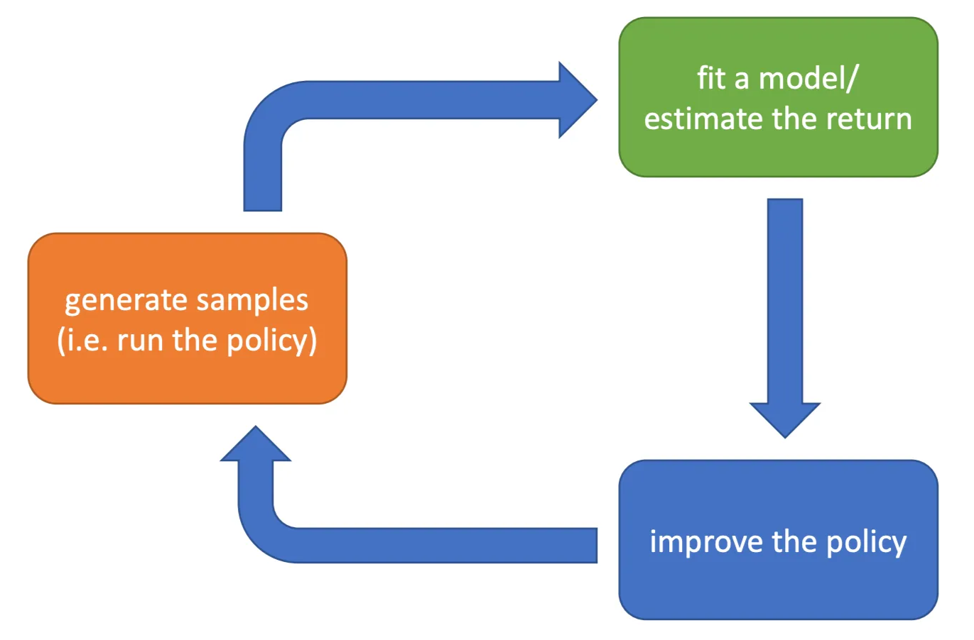
• Orange → $\frac{1}{N}\sum_{i=1}^N$
• Green → $\sum_{t=1}^Tr(\mathbf{s}_{i,t},\mathbf{a}_{i,t})$
• Blue → $\theta\leftarrow\theta+\alpha\nabla_{\theta}J(\theta)$

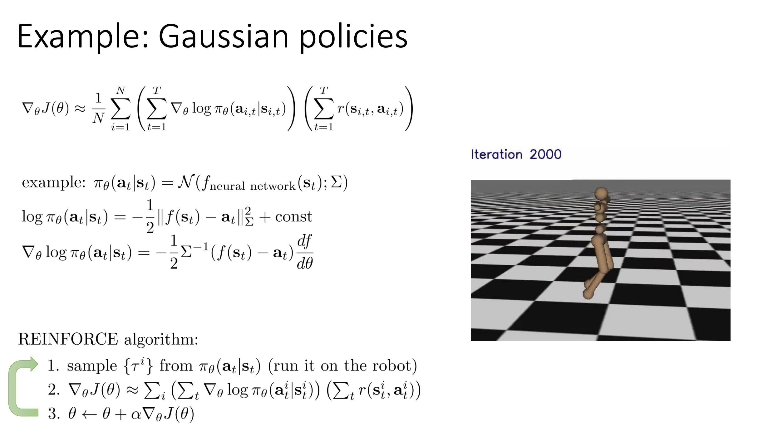
REINFORCE algorithm

1. sample ${\tau^i}$ from $\pi_\theta(\mathbf{a}_t^i | \mathbf{s}_t^i)$ ( run the policy )
2. $\nabla_\theta J(\theta)\approx\sum_i\left(\sum_t\nabla_\theta\log\pi_\theta(\mathbf{a}_t^i|\mathbf{s}_t^i)\right)\left(\sum_tr(\mathbf{s}_t^i,\mathbf{a}_t^i)\right)$
3. $\theta\leftarrow\theta+\alpha\nabla_{\theta}J(\theta)$

Understanding Policy Gradient

The maximum likelihood objective, which is a supervised learning objective, is given as

$$ \nabla_{\theta}J_{\mathrm{ML}}(\theta)\approx\frac{1}{N}\sum_{i=1}^{N}\left(\sum_{t=1}^{T}\nabla_{\theta}\log\pi_{\theta}(\mathbf{a}_{i,t}|\mathbf{s}_{i,t})\right) $$

In that case, we assume that the data $\mathbf{a}_{i,t}$ are good actions; while in Policy Gradient, it’s not necessary true, because we generated those actions by running our own previous policy. So the maximum likelihood gradient simply increases the $\log$ probabilities of all the actions, while the policy gradient might increase or decrease them depending on the values of their rewards — high reward trajectories get their $\log$ probabilities increased, low reward trajectories get their $\log$ probabilities decreased.

Sum up a little bit

• good stuff is made more likely
• bad stuff is made less likely
• simply formalizes the notion of “trial and error”

Partial observability

The main difference between states and observations is that the states satisfy the Markov property, whereas observations, in general, do not.

But when we derive the policy gradient, at no point did we actually use the Markov property, which means that we can use the policy gradients in partially observed MDPs without any modification.

What is wrong with the policy gradient?

For example, if we are given a policy

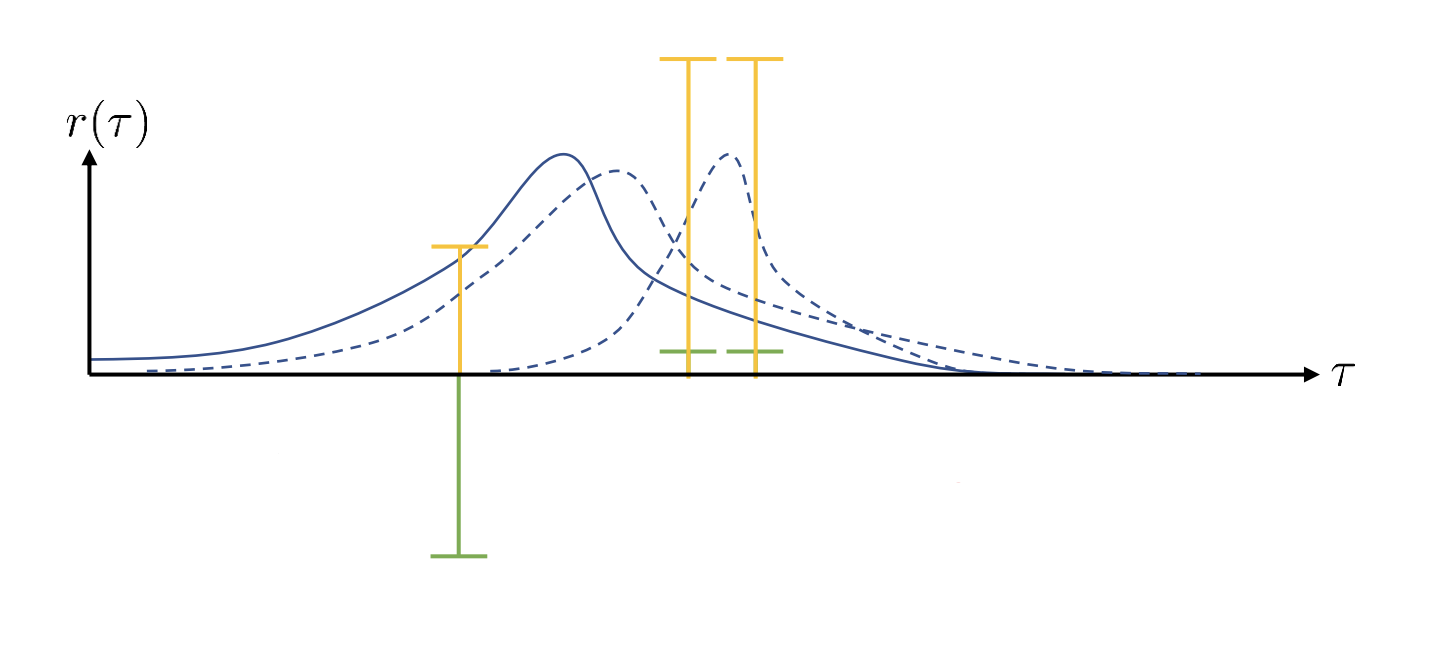
where the blue curve stands for the probabilities and the green curve stands for the rewards.

Clearly, in a policy gradient method, the blue curve temps to move right to increase the sum of rewards. Theoretically, the result shouldn’t change if we simply offset the rewards by a constant ( the yellow curve ). But in this case, the policy gradient method wants to increase the probabilities of both three samples and the policy ends up different from the previous one.

It’s actually an instance of high variance. Essentially, the policy gradient estimator has very high variance in terms of the samples that you get. So with different samples, you might end up with very different values of the policy gradient.

Reducing Variance

Causality: policy at time $t^{\prime}$ cannot affect reward at time $t$ when $t \lt t^{\prime}$.

We can use this assumption to reduce the variance. By doing so, we first rewrite the gradient function as

$$ \nabla_{\theta}J(\theta)\approx\frac{1}{N}\sum_{i=1}^{N}\sum_{t=1}^{T}\nabla_{\theta}\log\pi_{\theta}(\mathbf{a}_{i,t}|\mathbf{s}_{i,t})\left(\sum_{t^{\prime}=1}^{T}r(\mathbf{s}_{i,t^{\prime}},\mathbf{a}_{i,t^{\prime}})\right) $$

which means that, at every timestep, we multiply the gradient of $\log$ probability of the action at the time step $t$ by the sum of rewards of all timesteps in the past, present and future.

Therefore, what we are doing is changing the $\log$ probability of the action at every timestep based on whether that action corresponding to a large reward in the past, present and future. And yet we know the action at timestep $t$ can’t affect the rewards in the past, which means that the other rewards will necessarily have to cancel out that expectation. If we generate enough samples, eventually, we should see that all the rewards at time step $t^{\prime}\lt t$ will average out to a multiplier of $0$.

That’s how we modify the function

$$ \nabla_{\theta}J(\theta)\approx\frac{1}{N}\sum_{i=1}^{N}\sum_{t=1}^{T}\nabla_{\theta}\log\pi_{\theta}(\mathbf{a}_{i,t}|\mathbf{s}_{i,t})\left(\sum_{t^{\prime}=t}^{T}r(\mathbf{s}_{i,t^{\prime}},\mathbf{a}_{i,t^{\prime}})\right) $$

summing rewards from $t$ to $T$.

Now, having made that change, we actually end up with an estimator that has lower variance, since the totally sum is a smaller number. We can call the sum of rewards now as “reward to go”, denoted by $\hat{Q}_{i,t}$, and it’s actually a single-sample estimator of Q-function mentioned in the last lecture.

Baseline

What if the sum of rewards are all positive for every sample?

Intuitively, we want the policy gradient to increase the probabilities of trajectories that are better than average, and decrease the probabilities of trajectories that are worse than average.

$$ \nabla_{\theta}J(\theta)\approx\frac{1}{N}\sum_{i=1}^{N}\nabla_{\theta}\log p_{\theta}(\tau)[r(\tau)-b], \text{where}\space b=\frac{1}{N}\sum_{i=1}^{N}r(\tau) $$

We can show that subtract a constant $b$ from the rewards in policy gradient won’t change the gradient in expectation, but only change the variance. Or in other words, subtracting a baseline is unbiased in expectation.

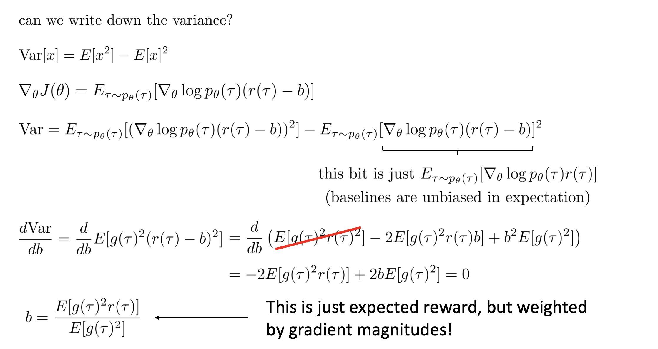
Analyzing variance

We actually can get the optimal baseline by mathematic.

Off-Policy Policy Gradients

Policy gradient is on-policy

On-policy means that when implementing REINFORCE algorithm, we must sample new samples from our policy every time the policy changed. This is problematic when doing deep reinforcement learning because neural networks only change a little bit with each gradient step, which might makes policy gradient very costly.

Therefore, on-policy learning can be extremely inefficient.

Off-policy learning & Importance sampling

What if we don’t have samples from $p_\theta({\tau})$? ( we have samples from some $\bar{p}(\tau)$ instead )

Importance sampling

$$ \begin{aligned} E_{x\thicksim p(x)}[f(x)] &= \int p(x)f(x)dx \ &= \int \frac{q(x)}{q(x)}p(x)f(x)dx \ &= \int q(x)\frac{p(x)}{q(x)}f(x)dx \ &= E_{x\thicksim q(x)}\left[\frac{p(x)}{q(x)}f(x)\right] \end{aligned} $$

Deriving the policy gradient with Importance sampling

Given parameters $\theta$, we can estimate the value of some new parameters $\theta^\prime$.

Using the Importance sampling, we have

$$ J(\theta^\prime) = E_{\tau\sim{p}_\theta(\tau)}[\frac{p_{\theta^\prime}(\tau)}{{p}_{\theta}(\tau)}r(\tau)] $$

Direct its differentiation, we have

$$ \nabla_{\theta^{\prime}}J(\theta^{\prime})=E_{\tau\sim p_{\theta}(\tau)}\left[\frac{\nabla_{\theta^{\prime}}p_{\theta^{\prime}}(\tau)}{p_{\theta}(\tau)}r(\tau)\right]=E_{\tau\sim p_{\theta}(\tau)}\left[\frac{p_{\theta^{\prime}}(\tau)}{p_{\theta}(\tau)}\nabla_{\theta^{\prime}}\log p_{\theta^{\prime}}(\tau)r(\tau)\right] $$

where, using the chain rule

$$ \frac{p_{\theta^\prime}(\tau)}{p_{\theta}(\tau)} = \frac{p(\mathbf{s}_1)\prod_{t=1}^{T}\pi_{\theta^\prime}(\mathbf{a}_t | \mathbf{s}_t)p(\mathbf{s}_{t+1}|\mathbf{s}_t, \mathbf{a}_t)}{p(\mathbf{s}_1)\prod_{t=1}^{T}\pi_{\theta}(\mathbf{a}_t | \mathbf{s}_t)p(\mathbf{s}_{t+1}|\mathbf{s}_t, \mathbf{a}_t)} = \frac{\prod_{t=1}^{T}\pi_{\theta ^\prime}(\mathbf{a}_t | \mathbf{s}_t)}{\prod_{t=1}^{T}\pi_{\theta}(\mathbf{a}_t | \mathbf{s}_t)} $$

If we substitute in, the differentiation will turn out to be

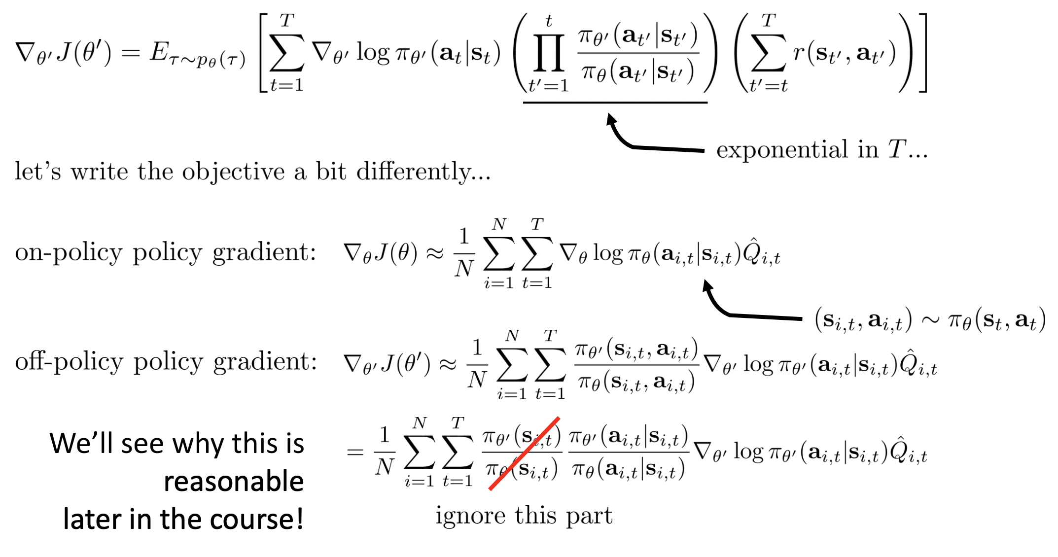
$$ \nabla_{\theta^{\prime}}J(\theta^{\prime})=E_{\tau\sim p_\theta(\tau)}\left[\left(\prod_{t=1}^T\frac{\pi_{\theta^{\prime}}(\mathbf{a}_t|\mathbf{s}_t)}{\pi_\theta(\mathbf{a}_t|\mathbf{s}_t)}\right)\left(\sum_{t=1}^T\nabla_{\theta^{\prime}}\log\pi_{\theta^{\prime}}(\mathbf{a}_t|\mathbf{s}_t)\right)\left(\sum_{t=1}^Tr(\mathbf{s}_t,\mathbf{a}_t)\right)\right] $$

But here we haven’t taken causality into consideration. We don’t need to consider the effect of current actions on the past rewards ( “reward to go” ). Further more, the future actions should not affect current weight.

$$ \nabla_{\theta^{\prime}}J(\theta^{\prime})= E_{\tau\sim p_\theta(\tau)}\left[\sum_{t=1}^T\nabla_{\theta^{\prime}}\log\pi_{\theta^{\prime}}(\mathbf{a}_t|\mathbf{s}_t)\left(\prod_{t^{\prime}=1}^t\frac{\pi_{\theta^{\prime}}(\mathbf{a}_{t^{\prime}}|\mathbf{s}_{t^{\prime}})}{\pi_\theta(\mathbf{a}_{t^{\prime}}|\mathbf{s}_{t^{\prime}})}\right)\left(\sum_{t^{\prime}=t}^Tr(\mathbf{s}_{t^{\prime}},\mathbf{a}_{t^{\prime}})\left(\prod_{t^{\prime\prime}=t}^{t^{\prime}}\frac{\pi_{\theta^{\prime}}(\mathbf{a}_{t^{\prime\prime}}|\mathbf{s}_{t^{\prime\prime}})}{\pi_\theta(\mathbf{a}_{t^{\prime\prime}}|\mathbf{s}_{t^{\prime\prime}})}\right)\right)\right] $$

If we ignore the last multiplication from $t$ to $t^{\prime}$, we will get a policy iteration algorithm, which will be covered more detailed in a future lecture.

A first-order approximation of IS ( preview )

Implementing Policy Gradients

Policy gradient with automatic differentiation

When we consider implementing policy gradients with following function

$$ \nabla_\theta J(\theta)\approx\frac{1}{N}\sum_{i=1}^N\sum_{t=1}^T\nabla_\theta\log\pi_\theta(\mathbf{a}_{i,t}|\mathbf{s}_{i,t})\hat{Q}_{i,t} $$

it is pretty inefficient to compute $\nabla_\theta\log\pi_\theta(\mathbf{a}_{i,t}|\mathbf{s}_{i,t})$ explicitly. So how can we compute policy gradients with automatic differentiation?

We need a graph such that its gradient is the policy gradient. Or in another word, we need to derive a potential function ( in mathematic, or loss/object function in machine learning ).

In particular, when comparing our function with maximum likelihood

$$ \nabla_{\theta} J_{\mathrm{ML}}(\theta) \approx \frac{1}{N}\sum_{i=1}^{N}\sum_{t=1}^{T}\nabla_{\theta} \log \pi_\theta(\mathbf{a}_{i,t} | \mathbf{s}_{i,t}) \ J_{\mathrm{ML}}(\theta) \approx \frac{1}{N}\sum_{i=1}^{N}\sum_{t=1}^{T}\log \pi_{\theta}(\mathbf{a}_{i,t} | \mathbf{s}_{i,t}) $$

we will find it extremely similar. Therefore, the trick here is to implement pseudo-loss as a weighted maximum likelihood

$$ \tilde{J}(\theta)\approx\frac{1}{N}\sum_{i=1}^N\sum_{t=1}^T\log\pi_\theta(\mathbf{a}_{i,t}|\mathbf{s}_{i,t})\hat{Q}_{i,t} $$

and $\nabla_{\theta}\tilde{J}(\theta)$ is exactly the gradient we want. ( $\hat{Q}_{i,t}$ need to be considered as a const here)

Here’s a pseudocode example in Tensorflow ( with discrete actions )

"""
maximum likelihood
"""
# Given:
# actions - (N * T) x Da tensor of actions
# states - (N * T) x Ds tensor of satets
# Build the graph:
logits = policy.predictions(states) # This should return (N * T) x Da tensor of action logits
negative_likelihoods = tf.nn.softmax_cross_entropy_with_logits(labels=actions, logits=logits)
loss = tf.reduce_mean(negative_likelihoods)
gradients = loss.gradients(loss, variables)

"""
policy gradient
"""
# Given:
# actions - (N * T) x Da tensor of actions
# states - (N * T) x Ds tensor of satets
# q_values - (N * T) x 1 tensor of estimated state-action values
# Build the graph:
logits = policy.predictions(states) # This should return (N * T) x Da tensor of action logits
negative_likelihoods = tf.nn.softmax_cross_entropy_with_logits(labels=actions, logits=logits)
weighted_negative_likelihoods = tf.multiply(negative_likelihoods, q_values)
loss = tf.reduce_mean(weighted_negative_likelihoods)
gradients = loss.gradients(loss, variables)

Policy gradient in practice

As we have mentioned before, the policy gradient has high variance, making it not as same as supervised learning. It means that the gradients might be really noisy. For example, in the first batch, the agent might get lucky and receive high rewards. The calculated gradient will point strongly in one direction. But in the second batch, the agent might be unlucky and receive low rewards even for similar actions. The calculated gradient might point in a completely opposite direction.

The most direct and classic method to combat high variance is considering using much larger batches. It’s based on the Central Limit Theorem ( or the Low of Large Numbers ) and is easy to understand. While tweaking learning rates can be very hard, since the agent might take a huge step based on a noisy gradient that happens to be wrong. Adaptive step size rules like ADAM can be OK-ish, for optimizers like ADAM maintain an adaptive learning rate for each parameter and consider the first moment ( momentum ) and second moment ( like variance ) of the gradients, which can, to some extent, smooth out the gradient noise, making it more stable than standard Stochastic Gradient Descent ( SGD ).