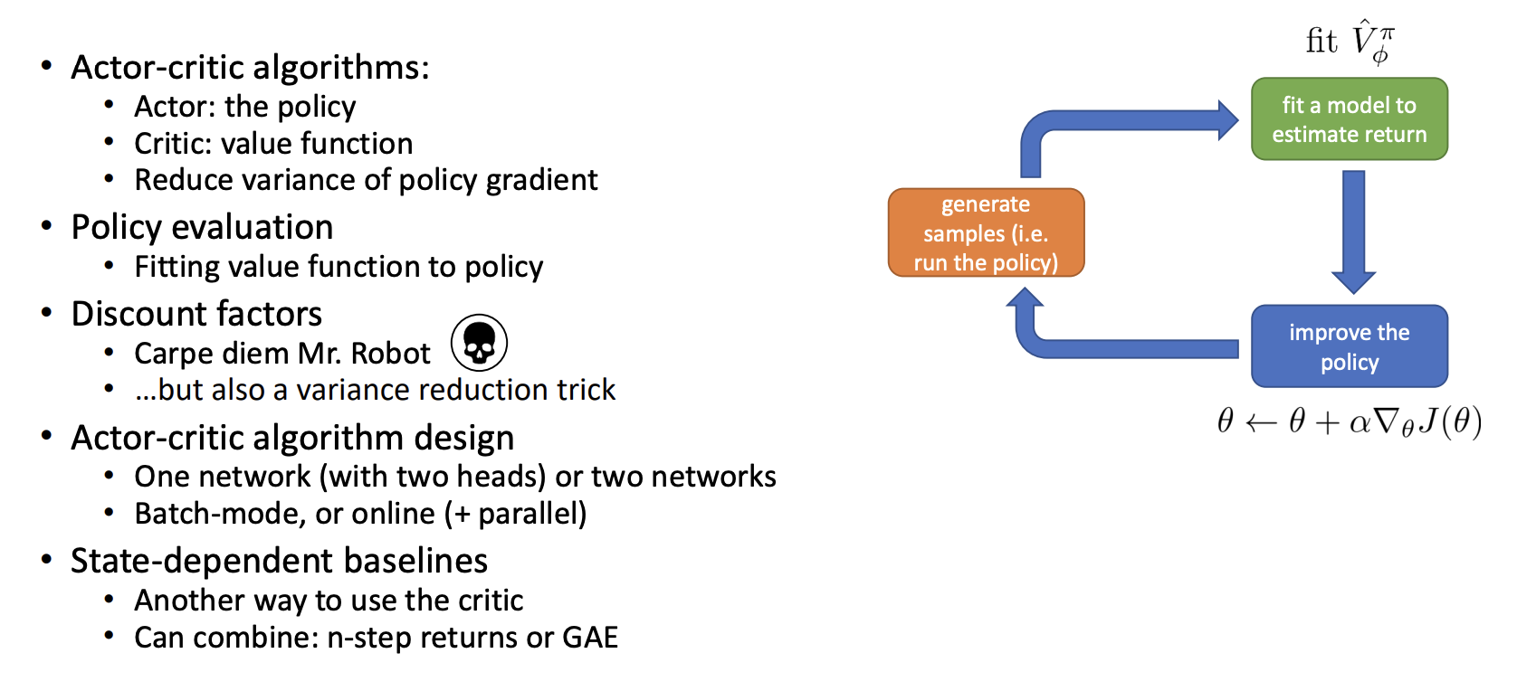
Lecture 6: Actor-Critic Algorithms

Lecture Slides & Videos

• Lecture 6: Actor-Critic Algorithms

• CS 285: Lecture 6, Part 1

• CS 285: Lecture 6, Part 2

• CS 285: Lecture 6, Part 3

• CS 285: Lecture 6, Part 4

• CS 285: Lecture 6, Part 5

Estimate Return

Recap: policy gradient

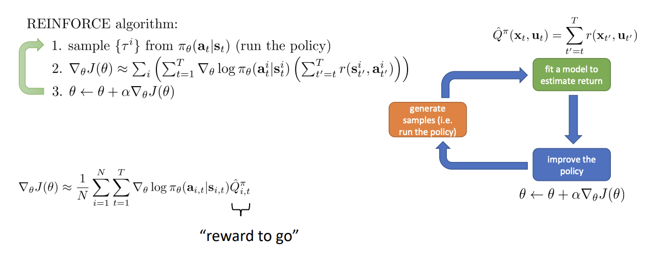
Improving the policy gradient

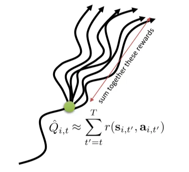
$\hat{Q}_{i,t}^{\pi} = \sum_{t^{\prime} = t}^{T}r(\mathbf{s}_{t^{\prime}}^i,\mathbf{a}_{t^{\prime}}^i)$ is the estimate of expected reward if we take action $\mathrm{a}_{i,t}$ in state $\mathrm{s}_{i,t}$. Can we get a better estimate?

Since the policy and the MDP ( Markov Decision Process ) have some randomness, even if we somehow accidentally land in the exactly same state $\mathrm{s}_{i,t}$ again and run the policy just like we did on the rollout, we might get a different outcome. This problem directly relates to the high variance of the policy gradient.

So we would have a better estimate of the reward-to-go if we could actually compute a full expectation over all these different possibilities.

$$ Q(\mathbf{s}_t, \mathbf{a}_t) = \sum_{t^{\prime} = t}^{T}E_{\pi_{\theta}}\left[r(\mathbf{s}_{t^{\prime}}, \mathbf{a}_{t^{\prime}}) | \mathbf{s}_t, \mathbf{a}_t \right] \ \nabla_{\theta} J(\theta)\approx\frac{1}{N}\sum_{i=1}^N\sum_{t=1}^T\nabla_{\theta}\log\pi_{\theta}(\mathbf{a}_{i,t}|\mathbf{s}_{i,t})Q({\mathbf{s}_{i,t}, \mathbf{a}_{i,t}}) $$

As mentioned in Lecture 5 we can give out a baseline that even lowers the variance further

$$ \nabla_{\theta}J(\theta)\approx\frac{1}{N}\sum_{i=1}^{N}\sum_{t=1}^{T}\nabla_{\theta}\log\pi_{\theta}(\mathbf{a}_{i,t}|\mathbf{s}_{i,t})(Q(\mathbf{s}_{i,t},\mathbf{a}_{i,t})-b) $$

where $b$ is an average reword. The question is, average what?

We can average $Q$ values, which is

$$ b_t=\frac{1}{N}\sum_iQ(\mathbf{s}_{i,t},\mathbf{a}_{i,t}) $$

It is reasonable, but it turns out that we can lower the variance even further because the baseline can depend on state, but it can’t depend on the action that leads to bias. So the better thing to do would be to compute the average reward over all the possibilities that start in that state, which is simply the definition of the value function.

$$ \nabla_{\theta} J(\theta)\approx\frac{1}{N}\sum_{i=1}^N\sum_{t=1}^T\nabla_{\theta}\log\pi_{\theta}(\mathbf{a}_{i,t}|\mathbf{s}_{i,t})\left(Q(\mathbf{s}_{i,t},\mathbf{a}_{i,t})-V(\mathbf{s}_{i,t})\right) \\ V(\mathbf{s}_t)=E_{\mathbf{a}_t\sim\pi_{\theta}(\mathbf{a}_t|\mathbf{s}_t)}[Q(\mathbf{s}_t,\mathbf{a}_t)] $$

In fact, we call the $Q(\mathbf{s}_{i,t},\mathbf{a}_{i,t})-V(\mathbf{s}_{i,t})$ the advantage function, for it represent how advantageous the action $\mathbf{a}_{i,t}$ is as compared to the average performance that we would expect the policy to get in the state $\mathbf{s}_{it}$.

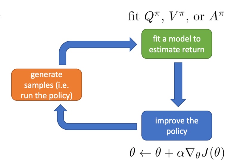
To sum up a little bit, we have following 3 functions

• $Q^\pi(\mathbf{s}_t,\mathbf{a}_t)=\sum_{t^{\prime}=t}^TE_{\pi_{\theta}}\left[r(\mathbf{s}_{t^{\prime}},\mathbf{a}_{t^{\prime}})|\mathbf{s}_t,\mathbf{a}_t\right]$ : total reword from taking $\mathbf{a}_t$ in $\mathbf{s}_t$
• $V^\pi(\mathbf{s}_t)=E_{\mathbf{a}_t\sim\pi_{\theta}(\mathbf{a}_t|\mathbf{s}_t)}[Q^\pi(\mathbf{s}_t,\mathbf{a}_t)]$ : total reward from $\mathbf{s}_t$
• $A^\pi(\mathbf{s}_t,\mathbf{a}_t)=Q^\pi(\mathbf{s}_t,\mathbf{a}_t)-V^\pi(\mathbf{s}_t)$ : how much better $\mathbf{a}_t$ is

Of cause, in reality, we won’t have the correct value of the advantage and we have to estimate it. Apparently, the better our estimate of the advantage, the lower the variance will be.

Value function fitting

Now we have a much more elaborate green box. The green box now involve fitting some kind of estimator, either an estimator to $Q^{\pi}$, $V^{\pi}$ or $A^{\pi}$.

So the question here is: fit what to what?

$$ \begin{aligned} Q^\pi(\mathbf{s}_t,\mathbf{a}_t) & =r(\mathbf{s}_t,\mathbf{a}_t)+\sum_{t^{\prime}=t+1}^{T}E_{\pi_{\theta}}\left[r(\mathbf{s}_{t^{\prime}},\mathbf{a}_{t^{\prime}})|\mathbf{s}_t,\mathbf{a}_t\right] \ & =r(\mathbf{s}_t,\mathbf{a}_t)+E_{\mathbf{s}_{t+1}\sim p(\mathbf{s}_{t+1}|\mathbf{s}_t,\mathbf{a}_t)}[V^{\pi}(\mathbf{s}_{t+1})] \ & \approx r(\mathbf{s}_t,\mathbf{a}_t)+V^\pi(\mathbf{s}_{t+1})\end{aligned} $$

Through above approximation, we can get a very appealing expression

$$ A^\pi(\mathbf{s}_t,\mathbf{a}_t)\approx r(\mathbf{s}_t,\mathbf{a}_t)+V^\pi(\mathbf{s}_{t+1})-V^\pi(\mathbf{s}_t) $$

This expression is appealing because the advantage equation is now depends entirely on $V$, which is more convenient to learn than $Q$ or $A$, since $Q$ and $A$ both depend on the state and the action whereas $V$ depends only on the state.

Maybe what we should do is just fit $V^{\pi}(\mathbf{s})$ ( so far ).

Policy evaluation

The process of fitting $V^{\pi}(\mathbf{s})$ is sometimes referred to as policy evaluation.

In fact, the objective function can be expressed as

$$ J(\theta) = E_{\mathbf{s_1} \sim p(\mathbf{s}_1)}\left[V^{\pi}(\mathbf{s}_1)\right] $$

So how can we perform policy evaluation?

A possible way is to implement Monte Carlo policy evaluation, which is what policy gradient does, by summing together the rewards along a trajectory starting at $\mathbf{s}_t$

$$ V^{\pi}(\mathbf{s}_t) \approx \sum_{t^{\prime} = t}^{T}r(\mathbf{s}_{t^{\prime}}, \mathbf{a}_{t^\prime}) $$

Ideally, what we would like to be able to do is sum over all possible trajectories that could occur when starting from $\mathbf{s}_t$, because there is more than one possibility, which is

$$ V^{\pi}(\mathbf{s}_t) \approx \frac{1}{N}\sum_{i=1}^{N}\sum_{t^{\prime} = t}^{T}r(\mathbf{s}_{t^{\prime}}, \mathbf{a}_{t^\prime}) $$

But this is generally impossible, because this requires us to be able to reset back to $\mathbf{s}_t$ and run multiple trials starting from that state. Generally, we don’t assume that we are able to do this. We only assume that we are able to run multiple trials from the initial states.

Monte Carlo evaluation with function approximation

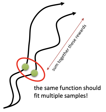
What happen if we use a neural network function approximator for the value function with this kind of Monte Carlo evaluation scheme?

Basically, we have a neural network $\hat{V}^{\pi}$ with parameter $\phi$. At every state, we are going to sum together the remaining rewards and that will produce our target values. But than, instead of plugging those reward to go directly into our policy gradient, we will actually fit a neural network to those values, and that will actually reduce our variance because even though we can’t visit the same state twice, our function approximator, as a neural network, will actually realize that different states that we visit in different trajectories are similar to one another.

As an example, even though the green state along the first trajectory will never be visited more than once in continuous state spaces, if we have another trajectory rollout that is kind of nearby, the function approximator will realize that theses two states are similar. When it tries to estimate the value at both of these states, the value of one will sort of leak into the value of the other.

That is essentially the generalization. Generalization means that your function approximator understands that nearby states should take on similar values.

• training data: $$ \left(\mathbf{s}_{i,t},\sum_{t^{\prime}=t}^Tr(\mathbf{s}_{i,t^{\prime}},\mathbf{a}_{i,t^{\prime}})\right), y_{i,t} =\sum_{t^{\prime}=t}^Tr(\mathbf{s}_{i,t^{\prime}},\mathbf{a}_{i,t^{\prime}}) $$
• supervised regression: $\mathcal{L}(\phi)=\frac{1}{2}\sum_i\left|\hat{V}_{\phi}^\pi(\mathbf{s}_i)-y_i\right|^2$

Can we do even better?

• ideal target: $y_{i,t}=\sum_{t^{\prime}=t}^TE_{\pi_{\theta}}[r(\mathbf{s}_{t^{\prime}},\mathbf{a}_{t^{\prime}})|\mathbf{s}_{i,t}]$
• Monte Carlo target: $y_{i,t}=\sum_{t^{\prime}=t}^Tr(\mathbf{s}_{i,t^{\prime}},\mathbf{a}_{i,t^{\prime}})$

If we again brake down the expected reward into the sum of the reward of the current timestep and the expected reward starting from the next time step

$$ y_{i,t}\approx r(\mathbf{s}_{i,t},\mathbf{a}_{i,t})+V^{\pi}(\mathbf{s}_{i,t+1})\approx r(\mathbf{s}_{i,t},\mathbf{a}_{i,t})+\hat{V}_{\phi}^{\pi}(\mathbf{s}_{i,t+1}) $$

that means we are going to approximate $V^{\pi}(\mathbf{s}_{i,t+1})$ using our function approximator.

• training data: $$ \left(\mathbf{s}_{i,t},r(\mathbf{s}_{i,t},\mathbf{a}_{i,t})+\hat{V}_{\phi}^{\pi}(\mathbf{s}_{i,t+1})\right) $$

where we will directly use previous fitted value function to estimate $\hat{V}_{\phi}^{\pi}(\mathbf{s}_{i,t+1})$. Sometimes, this is referred to as a bootstrapped estimate. With this improved method, the agent doesn’t have to wait for the episode to finish. It can create a training sample after each step. It’s a trade-off between lower variance and higher bias.

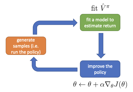
From Evaluation to Actor Critic

An actor-critic algorithm

Batch actor-critic algorithm:

1. sample ${ \mathbf{s}_i, \mathbf{a}_i }$ from $\pi_{\theta}(\mathbf{a} | \mathbf{s})$ ( run it on the robot )
2. fit $\hat{V}_{\phi}^{\pi}(\mathbf{s})$ to sampled reward sums
3. evaluate $\hat{A}^{\pi}(\mathbf{s}_i, \mathbf{a}_i) = r(\mathbf{s}_i, \mathbf{a}_i) + \hat{V}^{\pi}_{\phi}(\mathbf{s}_{i}^\prime) - \hat{V}^\pi_{\phi}(\mathbf{s}_i)$
4. $\nabla_{\theta} J(\theta) \approx \sum_i \nabla_{\theta} \log \pi_{\theta}(\mathbf{a}_i | \mathbf{s}_i) \hat{A}^\pi(\mathbf{s}_i, \mathbf{a}_i)$
5. $\theta \leftarrow \theta + \alpha \nabla_{\theta} J(\theta)$

Aside: discount factors

What if $T$ ( episode length ) is $\infin$? ( episodic tasks vs continuous/cyclical tasks )

→ $\hat{V}_{\phi}^{\pi}$ can get infinitely large in many cases

In that case, a simple trick is: better to get rewards sooner than later. So instead of setting target value to be $y_{i,t} \approx r(\mathbf{s}_{i,t},\mathbf{a}_{i,t})+\hat{V}_{\phi}^{\pi}(\mathbf{s}_{i,t+1})$, we use

$$ y_{i,t}\approx r(\mathbf{s}_{i,t},\mathbf{a}_{i,t})+\gamma\hat{V}_{\phi}^\pi(\mathbf{s}_{i,t+1}) $$

where $\gamma \in$ is called a discount factor ( 0.99 works well ).

The discount factor $\gamma$ actually changes the MDP. When adding the discount factor, we are adding a death state and we have a probability of $1-\gamma$ of transitioning to that death state at every time step. Once we enter the death state we never leave, so there’s no resurrection in this MDP, and the reward in the death state is always zero.

We can introduce the discount factor into regular Monte Carlo policy gradient.

• Option 1: reward-to-go

  $$ \nabla_{\theta} J(\theta)\approx\frac{1}{N}\sum_{i=1}^N\sum_{t=1}^T\nabla_{\theta}\log\pi_{\theta}(\mathbf{a}_{i,t}|\mathbf{s}_{i,t})\left(\sum_{t^{\prime}=t}^T\gamma^{t^{\prime}-t}r(\mathbf{s}_{i,t^{\prime}},\mathbf{a}_{i,t^{\prime}})\right) $$

• Option 2: original version

  $$ \begin{aligned} \nabla_{\theta} J(\theta) & \approx\frac{1}{N}\sum_{i=1}^N\left(\sum_{t=1}^T\nabla_{\theta}\log\pi_{\theta}(\mathbf{a}_{i,t}|\mathbf{s}_{i,t})\right)\left(\sum_{t=1}^T\gamma^{t-1}r(\mathbf{s}_{i,t^{\prime}},\mathbf{a}_{i,t^{\prime}})\right) \\ & = \begin{aligned} \frac{1}{N}\sum_{i=1}^{N}\sum_{t=1}^{T}\gamma^{t-1}\nabla_{\theta}\operatorname{log}\pi_{\theta}(\mathbf{a}_{i,t}|\mathbf{s}_{i,t})\left(\sum_{t^{\prime}=t}^{T}\gamma^{t^{\prime}-t}r(\mathbf{s}_{i,t^{\prime}},\mathbf{a}_{i,t^{\prime}})\right) \end{aligned}\end{aligned} $$

  In this case, because of the discount, not only do we care less about rewards further in the future, but also we care less about the decisions further in the future. As a result, we actually discount the gradient at every timestep by $\gamma^{t-1}$.

  However, in reality, this is not often quite what we want.

Basically, we do want a policy that does the right thing at every time step, not just in the early time steps. Another reason is that, the discount factor serves to reduce the variance of the policy gradient. By ensuring the reward sums are finite by putting a discount, we are also reducing variance at the cost of introducing bias by not accounting for all those rewards in the future.

Therefore, with critic, the policy gradient turns out to be

$$ \nabla_{\theta} J(\theta)\approx\frac{1}{N}\sum_{i=1}^N\sum_{t=1}^T\nabla_{\theta}\log\pi_{\theta}(\mathbf{a}_{i,t}|\mathbf{s}_{i,t})\left(r(\mathbf{s}_{i,t},\mathbf{a}_{i,t})+\gamma\hat{V}_{\phi}^\pi(\mathbf{s}_{i,t+1})-\hat{V}_{\phi}^\pi(\mathbf{s}_{i,t})\right) $$

and the step 3 in the batch actor-critic algorithm turns out to be

1. evaluate $\hat{A}^{\pi}(\mathbf{s}_i, \mathbf{a}_i) = r(\mathbf{s}_i, \mathbf{a}_i) + \gamma \hat{V}^{\pi}_{\phi}(\mathbf{s}_i^\prime) - \hat{V}^\pi_{\phi}(\mathbf{s}_i)$

One of the thing we can do with actor-critic algorithms, once we take them into the infinite horizon setting, is actually we can actually derive a fully online actor critic method. Instead of using policy gradients in a kind of episodic batch mode setting, where we collect a batch of trajectories, each trajectory runs all the way to the end and we use that to evaluate the gradient and update our policy, we could also have an online version where every single time step we update our policy.

Online actor-critic algorithm:

1. take action $\mathbf{a} \sim \pi_{\theta}(\mathbf{a} | \mathbf{s})$ , get $(\mathbf{s}, \mathbf{a}, \mathbf{s}^{\prime}, r)$
2. update $\hat{V}^{\pi}_{\phi}$ using target $r + \gamma \hat{V}^{\pi}_{\phi}(\mathbf{s}^{\prime})$
3. evaluate $\hat{A}^{\pi}(\mathbf{s}, \mathbf{a}) = r(\mathbf{s}, \mathbf{a}) + \gamma \hat{V}^{\pi}_{\phi}(\mathbf{s}^\prime) - \hat{V}^\pi_{\phi}(\mathbf{s})$
4. $\nabla_{\theta} J(\theta)\approx\nabla_{\theta}\log\pi_{\theta}(\mathbf{a}|\mathbf{s})\hat{A}^\pi(\mathbf{s},\mathbf{a})$
5. $\theta \leftarrow \theta + \alpha \nabla_{\theta} J(\theta)$

Actor-Critic Design Decisions

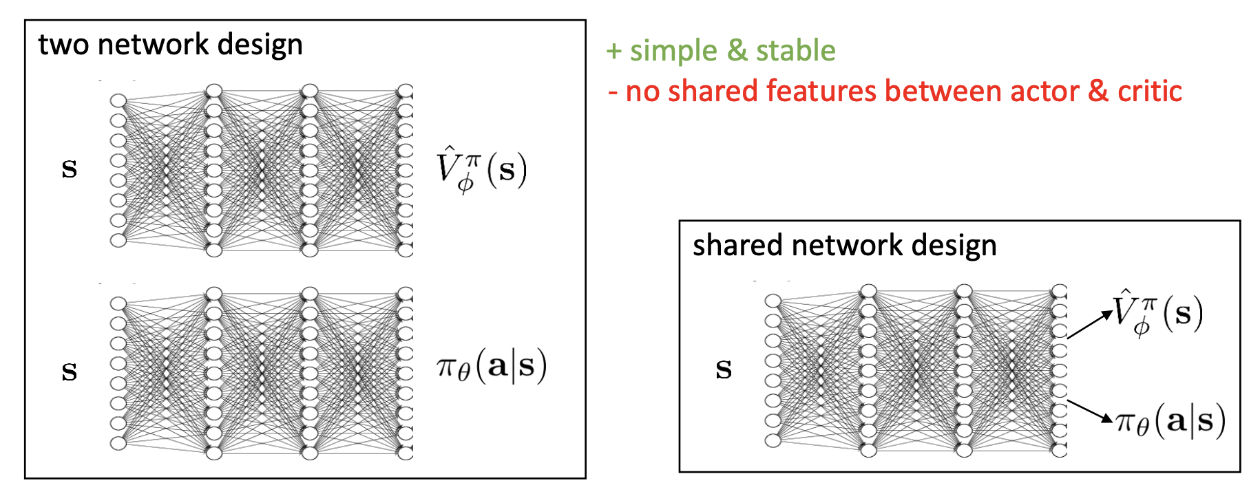
Architecture design

Basically, we can use a two network design: one maps a state $\mathbf{s}$ to $\hat{V}^\pi_{\phi}(\mathbf{s})$ and the other one maps $\mathbf{s}$ to $\pi_{\theta}(\mathbf{a} | \mathbf{s})$ . It’s a simple and stable design, but there is no shared features between actor & critic.

There is also a shared network design, where we have one trunk with separate heads, one for the value and one for the policy action distribution. In this case, the two heads share the internal representations so that, for example, if the value function figures out good representations first, the policy could benefit from them. This shared network design is a little bit harder to train because those shared layers are getting hit with very different gradients. The gradients from the value regression and the gradients from the policy will be on different scales and have different statistics and therefore require more hyper parameter tuning in order to stabilize this approach.

Online actor-critic in practice

The algorithm described above is fully online, meaning that it learns one sample at a time. Using just one sample to update deep neural nets with stochastic gradient descent will cause too much variance. These updates will all work best if we have a batch, for example, using parallel workers. In practice, the asynchronous parallel pattern is used more often.

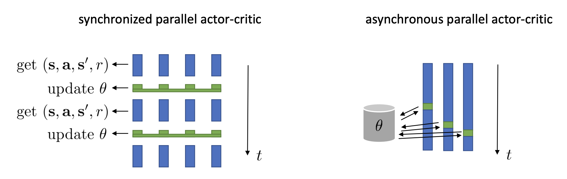
Can we remove the on-policy assumption entirely?

In the asynchronous actor-critic algorithm, the whole point is that we are able to use transitions that are generated by slightly older actors. If we can somehow get a way with using transitions that that are generated by much older actor, then maybe we don’t even need multiple threads by using older transitions from a same actor, a history. That is the off-policy actor-critic algorithm.

When updating the network, we’re going to use a replay buffer of all transitions we’ve seen, and load the batch from it. So we’re actually not going to necessarily use the latest transitions. But in this case, we have to modify our algorithm a bit since the batch that we load in from the buffer definitely comes from much older policies.

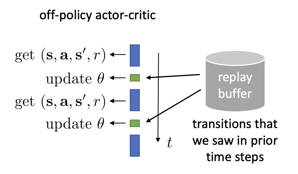
Online actor-critic algorithm:

1. take action $\mathbf{a} \sim \pi_{\theta}(\mathbf{a} | \mathbf{s})$, get $(\mathbf{s}, \mathbf{a}, \mathbf{s}^\prime, r)$, store in $\mathcal{R}$
2. sample a batch $(\mathbf{s}_i, \mathbf{a}_i, r_i, \mathbf{s}_i^\prime)$ from buffer $\mathcal{R}$
3. update $\hat{V}^{\pi}_{\phi}$ using target $y_i = r + \gamma \hat{V}^{\pi}_{\phi}(\mathbf{s}_i^{\prime})$ for each $\mathbf{s}_i$, with loss function as $\mathcal{L}(\phi)=\frac{1}{N}\sum_i\left|\hat{V}_{\phi}^\pi(\mathbf{s}_i)-y_i\right|^2$
4. evaluate $\hat{A}^{\pi}(\mathbf{s}_i, \mathbf{a}_i) = r(\mathbf{s}_i, \mathbf{a}_i) + \hat{V}^{\pi}_{\phi}(\mathbf{s}_i^\prime) - \hat{V}^\pi_{\phi}(\mathbf{s}_i)$
5. $\nabla_{\theta} J(\theta) \approx \frac{1}{N} \sum_i \nabla_{\theta} \log \pi_{\theta}(\mathbf{a}_i | \mathbf{s}_i) \hat{A}^\pi(\mathbf{s}_i, \mathbf{a}_i)$
6. $\theta \leftarrow \theta + \alpha \nabla_{\theta} J(\theta)$

But this algorithm is broken.

• $y_i = r + \gamma \hat{V}^{\pi}_{\phi}(\mathbf{s}_i^{\prime})$: $\mathbf{a}_i$ did not come from the latest $\pi_{\theta}$ , so $\mathbf{s}_i^\prime$ is also not the result of taking an action with the latest actor, which means that the target value is incorrect.
• $\nabla_{\theta} \log \pi_{\theta}(\mathbf{a}_i | \mathbf{s}_i)$: When computing the policy gradient, we actually get actions that are sampled from our policy because this needs to by an expected value under $\pi_{\theta}$. Otherwise, we need to employ some kind of correction such as importance sampling.

Fixing the value function

For the target value problem, we learn $\hat{Q}^\pi_{\phi}$ instead, because there is no assumption that $\mathbf{a}_i$ comes from the latest policy. So the Q-function is a valid function for any action.

→ 3. update $\hat{Q}^\pi_{\phi}$ using target $y_i = r + \gamma \hat{V}^{\pi}_{\phi}(\mathbf{s}_i^{\prime})$ for each $\mathbf{s}_i$, $\mathbf{a}_i$

But where do we get $\hat{V}^{\pi}_{\phi}(\mathbf{s}_i^{\prime})$? The trick is using the following equation

$$ V^\pi(\mathbf{s}_t)=\sum_{t^{\prime}=t}^TE_{\pi_{\theta}}\left[r(\mathbf{s}_{t^{\prime}},\mathbf{a}_{t^{\prime}})|\mathbf{s}_t\right]=E_{\mathbf{a}\sim\pi(\mathbf{a}_t|\mathbf{s}_t)}[Q(\mathbf{s}_t,\mathbf{a}_t)] $$

So we can replace the $\hat{V}^{\pi}_{\phi}(\mathbf{s}_i^{\prime})$ with $\hat{Q}^\pi_{\phi}(\mathbf{s}_i^\prime, \mathbf{a}_i^\prime)$, where $\mathbf{a}_i^\prime$ is the action sampled from the latest policy $\pi_{\theta}$ at $\mathbf{s}_i^\prime$. So we’re actually exploiting the fact that we have functional access to our policy so we can ask our policy what it would have if it have found itself in the old state $\mathbf{s}_i^\prime$ even though that it never actually happened.

→ 3. update $\hat{Q}^\pi_{\phi}$ using target $y_i = r + \gamma \hat{Q}^\pi_{\phi}(\mathbf{s}_i^\prime, \mathbf{a}_i^\prime)$ for each $\mathbf{s}_i$, $\mathbf{a}_i$

Fixing the policy update

We will use the same trick, but this time for $\mathbf{a}_i$ rather than $\mathbf{a}_i^\prime$ . We sample $\mathbf{a}_i^\pi \sim \pi_{\theta}(\mathbf{a} | \mathbf{s}_i)$, which is what the policy would have done if it had been in the buffer state $\mathbf{s}_i$.

→ 5. $\nabla_{\theta} J(\theta) \approx \frac{1}{N} \sum_i \nabla_{\theta} \log \pi_{\theta}(\mathbf{a}_i^\pi | \mathbf{s}_i) \hat{A}^\pi(\mathbf{s}_i, \mathbf{a}_i^\pi)$

But in practice, we plug in our $\hat{Q}^\pi_{\phi}$ directly to the equation instead of using a baseline. In this way, it has higher variance. But this is acceptable here because we don’t need to interact with a simulator to sample these actions, so it’s actually very easy to lower our variance just by generating more samples of the actions without actually generating more sampled states.

As for $\mathbf{s}_i$ , which does not come from $p_{\theta}(\mathbf{s})$ , we just accept it as a source of bias. The intuition for why it’s not so bad is that ultimately we want the optimal policy on $p_{\theta}(\mathbf{s})$ , but we get the optimal policy on a broader distribution.

So we have arrived at a quite complete version:

1. take action $\mathbf{a} \sim \pi_{\theta}(\mathbf{a} | \mathbf{s})$, get $(\mathbf{s}, \mathbf{a}, \mathbf{s}^\prime, r)$, store in $\mathcal{R}$
2. sample a batch $(\mathbf{s}_i, \mathbf{a}_i, r_i, \mathbf{s}_i^\prime)$ from buffer $\mathcal{R}$
3. update $\hat{Q}^\pi_{\phi}$ using target $y_i = r + \gamma \hat{Q}^\pi_{\phi}(\mathbf{s}_i^\prime, \mathbf{a}_i^\prime)$ for each $\mathbf{s}_i$, $\mathbf{a}_i$
4. $\nabla_{\theta} J(\theta) \approx \frac{1}{N} \sum_i \nabla_{\theta} \log \pi_{\theta}(\mathbf{a}_i^\pi | \mathbf{s}_i) \hat{Q}^\pi_{\phi}(\mathbf{s}_i, \mathbf{a}^\pi_i)$ where $\mathbf{a}_i^\pi \sim \pi_{\theta}(\mathbf{a} | \mathbf{s}_i)$
5. $\theta \leftarrow \theta + \alpha \nabla_{\theta} J(\theta)$ Example practical algorithm.
   Soft Actor-Critic: Off-Policy Maximum Entropy Deep Reinforcement…

Critics as Baselines

Critics as state-dependent baselines

Actor-critic:

$$ \nabla_{\theta} J(\theta)\approx\frac{1}{N}\sum_{i=1}^N\sum_{t=1}^T\nabla_{\theta}\log\pi_{\theta}(\mathbf{a}_{i,t}|\mathbf{s}_{i,t})\left(r(\mathbf{s}_{i,t},\mathbf{a}_{i,t})+\gamma\hat{V}_{\phi}^\pi(\mathbf{s}_{i,t+1})-\hat{V}_{\phi}^\pi(\mathbf{s}_{i,t})\right) $$

• lower variance ( due to critic )
• not unbiased ( if the critic is not perfect )

Policy gradient:

$$ \begin{aligned}\nabla_{\theta} J(\theta)\approx\frac{1}{N}\sum_{i=1}^N\sum_{t=1}^T\nabla_{\theta}\log\pi_{\theta}(\mathbf{a}_{i,t}|\mathbf{s}_{i,t})\left(\left(\sum_{t^{\prime}=t}^T\gamma^{t^{\prime}-t}r(\mathbf{s}_{i,t^{\prime}},\mathbf{a}_{i,t^{\prime}})\right)-b\right)\end{aligned} $$

• no bias
• higher variance ( because single-sample estimate )

Can we use $\hat{V}_{\phi}^{\pi}$ and still keep estimator unbiased?

The answer is yes and the method is called critics as state-dependent baselines.

$$ \nabla_{\theta} J(\theta)\approx\frac{1}{N}\sum_{i=1}^N\sum_{t=1}^T\nabla_{\theta}\log\pi_{\theta}(\mathbf{a}_{i,t}|\mathbf{s}_{i,t})\left(\sum_{t^{\prime}=t}^T\gamma^{t^{\prime}-t}r(\mathbf{s}_{i,t^{\prime}},\mathbf{a}_{i,t^{\prime}}) - \hat{V}_{\phi}^{\pi}(\mathbf{s}_{i,t}) \right) $$

In this case, the variance is lowered because the baseline is closer to rewards. Also, it’s unbiased because $\hat{V}_{\phi}^{\pi} (\mathbf{s}_{i,t})$ only depends on state. It can be proved that the estimator is unbiased if the baseline $b$ only depends on state. Otherwise, if the baseline $b$ also depends on action, the estimator is biased.

Control variates: action-dependent baselines

What if the baseline $b$ depends on more things, which is both state and action? In that case, the variance supposes to be even lower. The method that use both state and action dependent baselines is called control variates.

We start with the advantage function

$$ A^\pi(\mathbf{s}_t, \mathbf{a}_t) = Q^\pi(\mathbf{s}_t, \mathbf{a}_t) - V^\pi(\mathbf{s}_t) $$

• state-dependent baselines
  • no bias
  • higher variance ( because single-sample estimate )

$$ \hat{A}^\pi(\mathbf{s}, \mathbf{a}) = \sum_{t^{\prime}=t}^T\gamma^{t^{\prime}-t}r(\mathbf{s}_{t^{\prime}},\mathbf{a}_{t^{\prime}}) - V_{\phi}^{\pi}(\mathbf{s}_t) $$

• action-dependent baselines
  • goes to zero in expectation if critics is correct
  • not correct

$$ \hat{A}^\pi(\mathbf{s}, \mathbf{a}) = \sum_{t^{\prime}=t}^T\gamma^{t^{\prime}-t}r(\mathbf{s}_{t^{\prime}},\mathbf{a}_{t^{\prime}}) - Q^\pi_{\phi}(\mathbf{s}_t,\mathbf{a}_t) $$

There is an error term we have to compensate for in the action-dependent baselines. So we arrive at this equation

$$ \begin{aligned}\nabla_{\theta} J(\theta)\approx\frac{1}{N}\sum_{i=1}^N\sum_{t=1}^T\nabla_{\theta}\log\pi_{\theta}(\mathbf{a}_{i,t}|\mathbf{s}_{i,t})\left(\hat{Q}_{i,t}-Q_{\phi}^\pi(\mathbf{s}_{i,t},\mathbf{a}_{i,t})\right)+ & \frac{1}{N}\sum_{i=1}^N\sum_{t=1}^T\nabla_{\theta} E_{\mathbf{a}\sim\pi_{\theta}(\mathbf{a}_t|\mathbf{s}_{i,t})}\left[Q_{\phi}^\pi(\mathbf{s}_{i,t},\mathbf{a}_t)\right]\end{aligned} $$

This equation is a valid estimator for the policy gradient even if the baseline doesn’t depend on the action, where in that case the second term basically vanishes.

The advantage of this estimator is that in many cases, the second term can actually be evaluated very accurately. If we have discrete actions, we can sum over all possible actions. If we have continuous actions, we can sample a very large number of actions because evaluating expectation of our actions doesn’t require sampling new states. So it doesn’t require actually interacting with the world.

Eligibility traces & n-step returns

Still we gonna start with the advantage estimator in an actor-critic algorithm, which we denote it as $\hat{A}_C^{\pi}$, with lower variance but higher bias if the value is wrong ( it always is )

$$ \hat{A}_C^{\pi}(\mathbf{s}_t, \mathbf{a}_t) = r(\mathbf{s}_t, \mathbf{a}_t) + \gamma \hat{V}^{\pi}_{\phi}(\mathbf{s}_t^\prime) - \hat{V}^\pi_{\phi}(\mathbf{s}_t) $$

and the Monte Carlo advantage estimator, which we denote it as with no bias but much higher variance because of the single sample estimation.

$$ \hat{A}_{MC}^\pi(\mathbf{s}_t, \mathbf{a}_t) = \sum_{t^{\prime}=t}^\infin\gamma^{t^{\prime}-t}r(\mathbf{s}_{t^{\prime}},\mathbf{a}_{t^{\prime}}) - \hat{V}_{\phi}^{\pi}(\mathbf{s}_t) $$

Can we combine these two, to control bias/variance tradeoff?

• When we are using a discount, the reward will decrease over time, which means that the bias gotten from the value function is much less of a problem if we put the value function out of the next time step but further in the future.

  

• On the other hand, the variance that we get from the single sample estimator is also much more of a problem further into the future. It’s quite natural to understand.

  

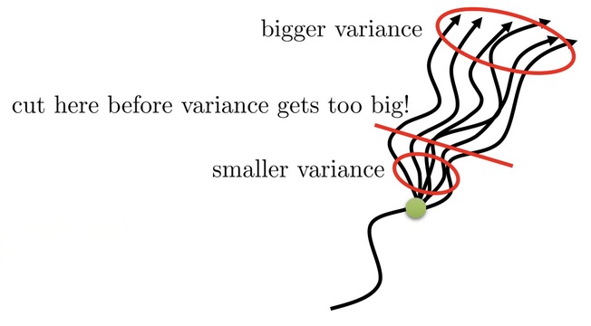
The way we gonna use to combine these is constructing a n-step returns estimator. In a n-step return estimator, we sum up rewards until some time step ends and cut it off to replace it with the value function. The advantage estimator will be something like this

$$ \hat{A}_n^\pi(\mathbf{s}_t,\mathbf{a}_t)=\sum_{t^{\prime}=t}^{t+n}\gamma^{t^{\prime}-t}r(\mathbf{s}_{t^{\prime}},\mathbf{a}_{t^{\prime}})-\hat{V}_{\phi}^\pi(\mathbf{s}_t)+\gamma^n\hat{V}_{\phi}^\pi(\mathbf{s}_{t+n}) $$

Generalized advantage estimation

Take a step further. We don’t need to choose just on $n$. We can construct a kind of fused estimator which we’re going to call $\hat{A}_{\mathrm{GAE}}^\pi$ for Generalized Advantage Estimation.

$$ \hat{A}_{\mathrm{GAE}}^\pi(\mathbf{s}_t,\mathbf{a}_t)=\sum_{n=1}^\infty w_n\hat{A}_n^\pi(\mathbf{s}_t,\mathbf{a}_t) $$

GAE consists of a weighted average of all possible n-step return estimators with a weight for different $n$. The way that we can choose the weight is by utilizing the insight that we’ll have more bias if we use small $n$ and more variance if we use large $n$. A decent choice that leads to an especially simple algorithm is to use an exponential falloff $w_n \propto \lambda^{n-1}$.

Therefore, the advantage estimation can then be written as

$$ \hat{A}^\pi_{GAE}(\mathbf{s}_t,\mathbf{a}_t) = r(\mathbf{s}_t, \mathbf{a}_t) + \gamma((1-\gamma)\hat{V}_{\phi}^{\pi}(\mathbf{s}_{t+1}) + \lambda(r(\mathbf{s}_{t+1}, \mathbf{a}_{t+1}) + \gamma((1-\lambda)\hat{V}_{\phi}^\pi(\mathbf{s}_{t+2}) + \lambda r(\mathbf{s}_{t+2}, \mathbf{a}_{t+2}) + …))) $$

or in a more elegant way

$$ \hat{A}^\pi_{GAE} (\mathbf{s}_t, \mathbf{a}_t) = \sum_{t^\prime = t}^\infin(\gamma\lambda)^{t^\prime - t}(\delta_{t^\prime}), \text{where} \space \delta_{t^{\prime}}=r(\mathbf{s}_{t^{\prime}},\mathbf{a}_{t^{\prime}})+\gamma\hat{V}_{\phi}^{\pi}(\mathbf{s}_{t^{\prime}+1})-\hat{V}_{\phi}^{\pi}(\mathbf{s}_{t^{\prime}}) $$

the $\delta_{t^\prime}$ here, known as TD-error ( Temporal Difference Error ), is like a single step advantage estimator, and the $(\gamma \lambda)$ has similar effect as discount.

Review, Examples, and Additional Readings