Lecture 7: Value Function Methods

Lecture Slides & Videos

• Lecture 7: Value Function Methods

• CS 285: Lecture 7, Part 1

• CS 285: Lecture 7, Part 2

• CS 285: Lecture 7, Part 3

• CS 285: Lecture 7, Part 4

Can we omit policy gradient completely?

This is possible since $A^{\pi}(\mathbf{s}_t,\mathbf{a}_t)$ actually indicates how better is $\mathbf{a}_t$ than the average action according to $\pi$ . So $\arg \max_{\mathbf{a}_t}A^\pi(\mathbf{s}_t, \mathbf{a}_t)$ suppose to be the best action from $\mathbf{s}_t$ if we then follow $\pi$ . How about we forget about policies, regardless of what $\pi(\mathbf{a}_t | \mathbf{s}_t)$ is and just use this action. In this case, the policy turns out to be

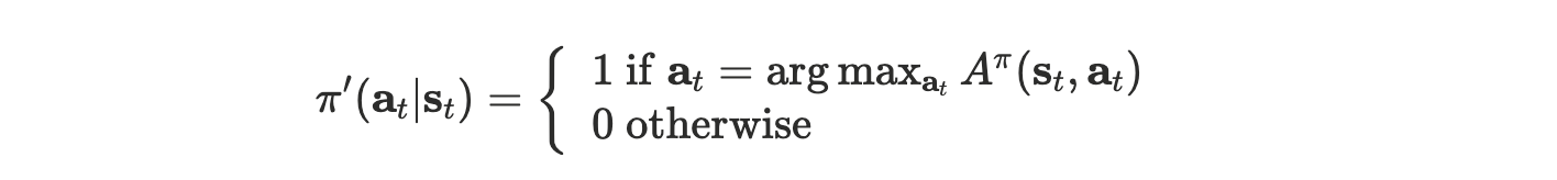
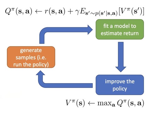
This is what we called policy iteration.

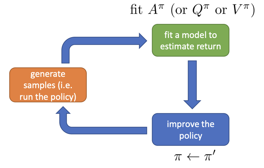
Policy iteration

Different from policy gradient, we fit some kind of value function that estimate the advantage in the green box and there won’t be any learning process in the blue box. We just set the policy to be the $\arg \max$ policy.

policy iteration algorithm:

1. evaluate $A^\pi(\mathbf{s}, \mathbf{a})$
2. set $\pi\leftarrow\pi^{\prime}$

The second step is pretty straight-forward. But how can we evaluate the advantage $A^{\pi}$?

As before, we can express the advantage as

$$ A^\pi(\mathbf{s},\mathbf{a})=r(\mathbf{s},\mathbf{a})+\gamma E[V^\pi(\mathbf{s}^{\prime})]-V^\pi(\mathbf{s}) $$

Again let try to evaluate $V^{\pi}(\mathbf{s})$.

Dynamic programming

One way to evaluate $V^{\pi}(\mathbf{s})$ is to use dynamic programming. Let’s assume we know $p(\mathbf{s}^{\prime}|\mathbf{s}, \mathbf{a})$, and $\mathbf{s}$ and $\mathbf{a}$ is both discrete ( and small ), which means can be represented in a tabular form. Here’s an example.

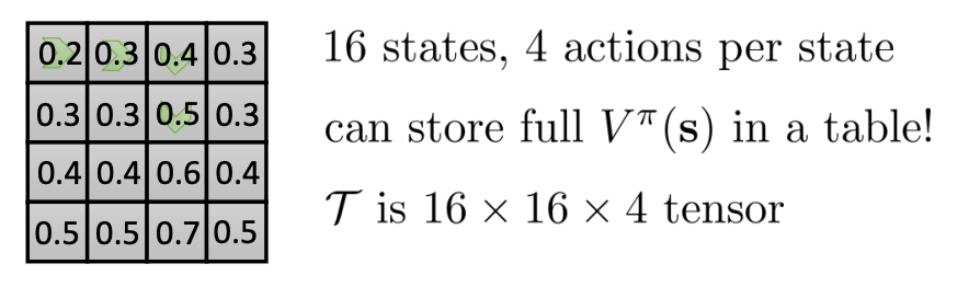
Now we can write down the bootstrapped update for the value function that we saw in Lecture 6 in terms of these explicit known probabilities.

$$ V^\pi(\mathbf{s})\leftarrow E_{\mathbf{a}\sim\pi(\mathbf{a}|\mathbf{s})}[r(\mathbf{s},\mathbf{a})+\gamma E_{\mathbf{s}^{\prime}\sim p(\mathbf{s}^{\prime}|\mathbf{s},\mathbf{a})}[V^\pi(\mathbf{s}^{\prime})]] $$

Of course we need to know $V^{\pi}(\mathbf{s}^\prime)$ so we’re going to use our current estimate of the value function.

What’s more, the second step of policy iteration indicates that our policy will be deterministic. So the expected value with respect to this $\pi$ can be simplified.

$$ V^\pi(\mathbf{s})\leftarrow r(\mathbf{s},\pi(\mathbf{s}))+\gamma E_{\mathbf{s}^{\prime}\sim p(\mathbf{s}^{\prime}|\mathbf{s},\pi(\mathbf{s}))}[V^\pi(\mathbf{s}^{\prime})] $$

Policy iteration with dynamic programming:

1. evaluate $V^{\pi}(\mathbf{s})$

   1. policy evaluation:

      $$ V^\pi(\mathbf{s})\leftarrow r(\mathbf{s},\pi(\mathbf{s}))+\gamma E_{\mathbf{s}^{\prime}\sim p(\mathbf{s}^{\prime}|\mathbf{s},\pi(\mathbf{s}))}[V^\pi(\mathbf{s}^{\prime})] $$

      repeat this recursion for multiple times eventually converges to a fixed point, which is the true value function $V^{\pi}$.

2. set $\pi\leftarrow\pi^{\prime}$

There’s even simpler dynamic programming method.

$$ A^\pi(\mathbf{s},\mathbf{a})=r(\mathbf{s},\mathbf{a})+\gamma E[V^\pi(\mathbf{s}^{\prime})]-V^\pi(\mathbf{s}) $$

If we remove the $- V^{\pi}(\mathbf{s})$, we just get the Q-function. Since we are taking the $\arg \max$ with respect to $\mathbf{a}$ , any term that doesn’t depend on actually doesn’t influence the result.

$$ \arg\max_{\mathbf{a}_t}A^\pi(\mathbf{s}_t,\mathbf{a}_t)=\arg\max_{\mathbf{a}_t}Q^\pi(\mathbf{s}_t,\mathbf{a}_t) \ Q^\pi(\mathbf{s},\mathbf{a})=r(\mathbf{s},\mathbf{a})+\gamma E[V^\pi(\mathbf{s}^{\prime})] $$

Right now, in the policy evaluation, the recursion is basically like this: pick $\arg\max_{\mathbf{a}_t}Q^\pi(\mathbf{s}_t,\mathbf{a}_t)$ → update the policy → calculate the new $Q^{\pi}(\mathbf{s}, \mathbf{a})$ → pick $\arg\max_{\mathbf{a}_t}Q^\pi(\mathbf{s}_t,\mathbf{a}_t)$.

We can skip the policy and compute values directly.

Value iteration algorithm:

1. set $Q(\mathbf{s}, \mathbf{a}) \leftarrow r(\mathbf{s},\mathbf{a}) + \gamma E[V(\mathbf{s}^\prime)]$
2. set $V(\mathbf{s}) \leftarrow \max_\mathbf{a}Q(\mathbf{s}, \mathbf{a})$

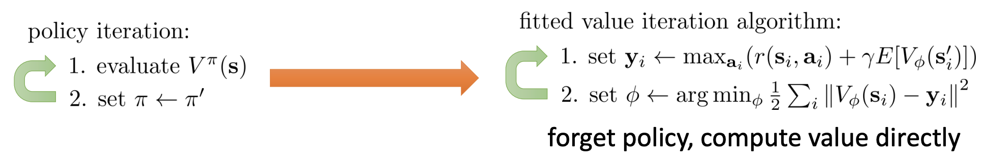
This procedure can be simplified even further if we actually take step 2 and plug it into step 1 to replace the value function in step 1.

Fitted Value Iteration & Q-Iteration

In most cases, maintaining a table over all the states is impossible for a discrete state space. For continuous state space, it’s actually just infinite and never possible. This is sometimes referred to as the curse of dimensionality. So we’ll use a function approximator, pretty similar to what we did in Lecture 6.

Fitted value iteration algorithm:

1. set $\mathbf{y}_i\leftarrow\max_{\mathbf{a}_i}(r(\mathbf{s}_i,\mathbf{a} _i)+\gamma E[V\phi(\mathbf{s}_i^{\prime})])$
2. set $\phi\leftarrow\arg\min_\phi\frac{1}{2}\sum_i\left|V_\phi(\mathbf{s}_i)-\mathbf{y}_i\right|^2$

What if we don’t know the transition dynamics?

There are two ways in which requires knowledge of the transition dynamics when implementing fitted value iteration algorithm.

• it requires being able to compute that expected value;
• it requires to be able to try multiple different actions from the same state ( which we can’t do in general if we can only run policies in the environment ).

Let’s go back to policy iteration, especially in policy evaluation:

$$ V^\pi(\mathbf{s})\leftarrow r(\mathbf{s},\pi(\mathbf{s}))+\gamma E_{\mathbf{s}^{\prime}\sim p(\mathbf{s}^{\prime}|\mathbf{s},\pi(\mathbf{s}))}[V^\pi(\mathbf{s}^{\prime})] $$

What if instead of applying the value function recurrence to learn the value function, we directly construct a Q-function recurrence in an analogous way.

$$ \begin{aligned}Q^\pi(\mathbf{s},\mathbf{a})\leftarrow r(\mathbf{s},\mathbf{a})+\gamma E_{\mathbf{s^{\prime}}\sim p(\mathbf{s^{\prime}}|\mathbf{s},\mathbf{a})}[Q^\pi(\mathbf{s^{\prime}},\pi(\mathbf{s^{\prime}}))]\end{aligned} $$

The subtle difference is very important because now as the policy $\pi$ changes, the action $\mathbf{a}$ I need to sample for $\mathbf{s}^\prime$ ( basically the $\mathbf{s}, \mathbf{a}$ on the right side of the conditioning bar ) doesn’t actually change. This means that if we have a bunch of samples $(\mathbf{s} , \mathbf{a}, \mathbf{s}^\prime, r)$, we can use those samples to fit the Q-function regardless of what policy we have.

It turns out that this very seemingly simple change allows us to perform policy iteration without actually knowing the transition dynamics just by sampling some $(\mathbf{s}, \mathbf{a}, \mathbf{s}^\prime, r)$ tuples which we can get by running any policy we want. This is the basis of most value-based model-free RL algorithms.

Can we do the “max” trick again?

We have used the “max” tick to turn the policy iteration into fitted value iteration algorithm:

In the fitted Q-iteration algorithm:

1. set $\mathbf{y}_i\leftarrow r(\mathbf{s}_i,\mathbf{a}_i)+\gamma E[V _\phi(\mathbf{s}_i^{\prime})] \leftarrow \text{approximate } E[V(\mathbf{s}_{i}^{\prime})]\approx\max_{\mathbf{a}^{\prime}}Q_{\phi}(\mathbf{s}_{i}^{\prime},\mathbf{a}_{i}^{\prime})$
2. set $\phi\leftarrow\arg\min_\phi\frac{1}{2}\sum_i\left|Q_\phi(\mathbf{s}_i,\mathbf{a}_i)-\mathbf{y}_i\right|^2$

The problem, as mentioned above, is that we have to evaluate step 1 without knowing the transition probabilities. So the first trick is that we’re going to replace $E[V_{\phi}(\mathbf{s}_i^\prime)]$ with $\max_{\mathbf{a}^\prime} Q_{\phi}(\mathbf{s}^\prime_i, \mathbf{a}_i^\prime)$ because we’re only approximating $Q_\phi$ instead of $V_\phi$ . The second trick is that instead of taking a full expectation over all possible next states, we’re going to use the samples.

• pros:
  • works even for off-policy samples (unlike actor-critic)
  • only one network, no high-variance policy gradient
• cons:
  • no convergence guarantees for non-linear function approximation ( more on this later )

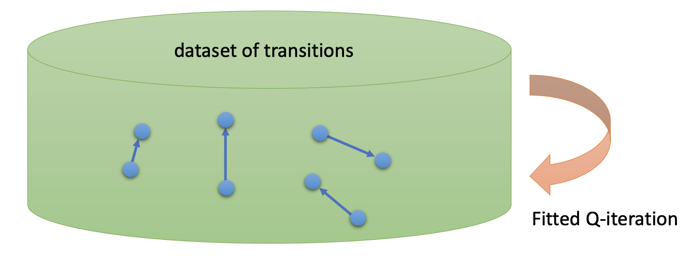
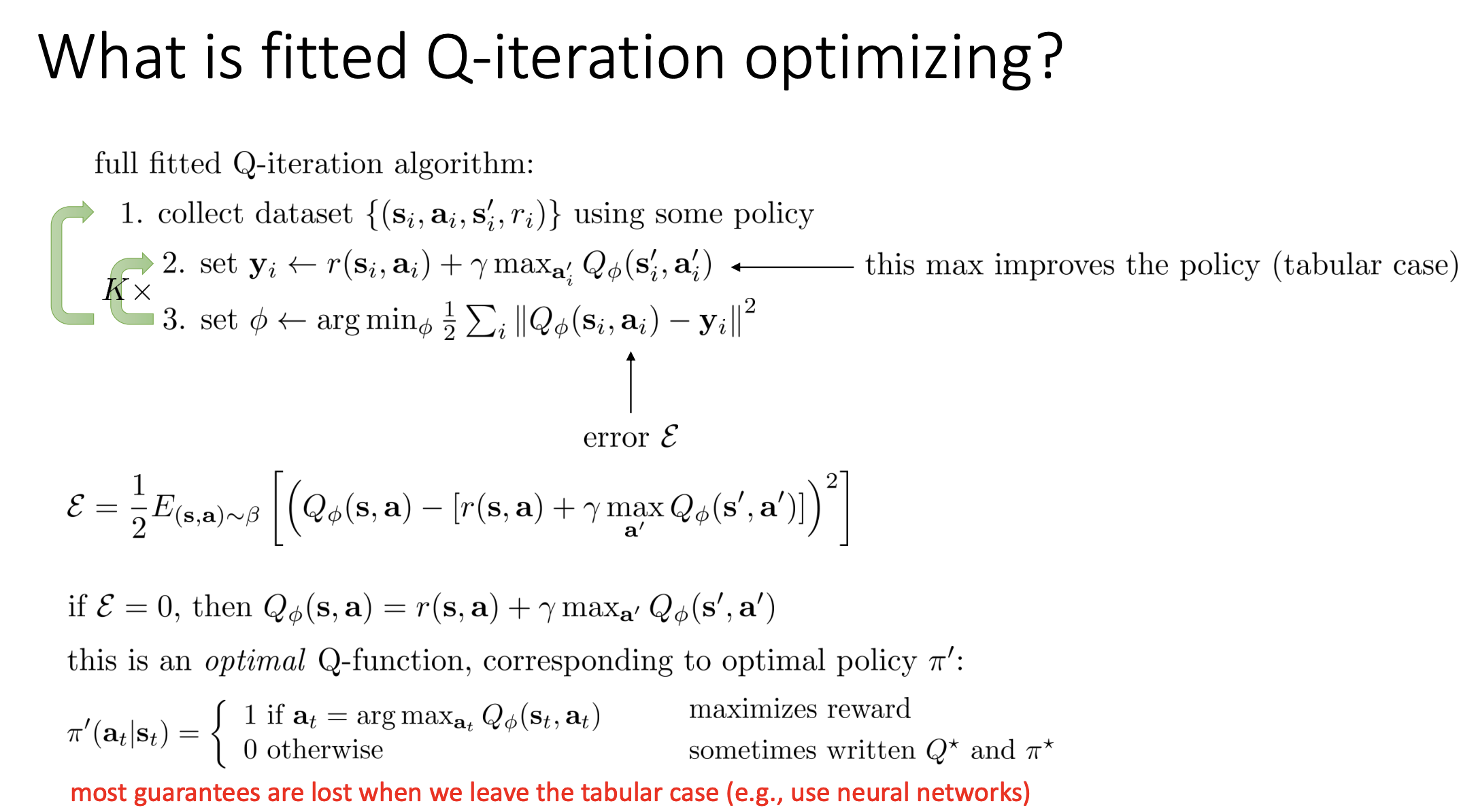
Full Fitted Q-iteration algorithm:

1. collect dataset $\left( \mathbf{s}_i, \mathbf{a}_i, \mathbf{s}_i^\prime, r_i \right)$ tuples using some policy
   1. dataset size $N$
   2. collection policy
2. set $\mathbf{y}_{i}\leftarrow r(\mathbf{s}_{i},\mathbf{a}_{i})+\gamma\max_{\mathbf{a}_{i}^{\prime}}Q_{\phi}(\mathbf{s}_{i}^{\prime},\mathbf{a}_{i}^{\prime})$
3. set $\phi\leftarrow\arg\min_\phi\frac{1}{2}\sum_i\left|Q_\phi(\mathbf{s}_i,\mathbf{a}_i)-\mathbf{y}_i\right|^2$
   1. a very common design for the neural network architecture for a Q-function with discrete actions is actually to have the actions being the outputs rather than inputs ( more on this later )
   2. gradient steps $S$
   3. iterations $K$ ( step 2 & 3 )

From Q-Iteration to Q-Learning

The full fitting Q-iteration algorithm is off-policy, which means that we do not need samples from the latest policy, typically we can take many gradient steps on the same set of samples or reuse samples from previous iterations.

Intuitively, the main reason that fitted Q-iteration allows us to use off-policy data is that the only one place where the policy is implicitly used is actually utilizing the Q-function rather than stepping through the simulator. As our policy changes, what really changes is $\max_{\mathbf{a}_{i}^{\prime}}Q_{\phi}(\mathbf{s}_{i}^{\prime},\mathbf{a}_{i}^{\prime})$ . The way we got this $\max$ is by taking the $\arg \max$, which is our policy, and then plugging it back into the Q-value. Conveniently enough, it shows up as an argument to the Q-function which means that as the policy changes, as the action $\mathbf{a}_i^\prime$ changes, we do not need to generate new rollouts.

One way we can think of fitted Q-iteration is that we have a big bucket of different transitions and what we’ll do is that we’ll back up the values along each of the transitions and each of those backups will improve our Q-value. We don’t really care so much about which specific transitions they are as long as they can cover the space of all possible transitions quite well.

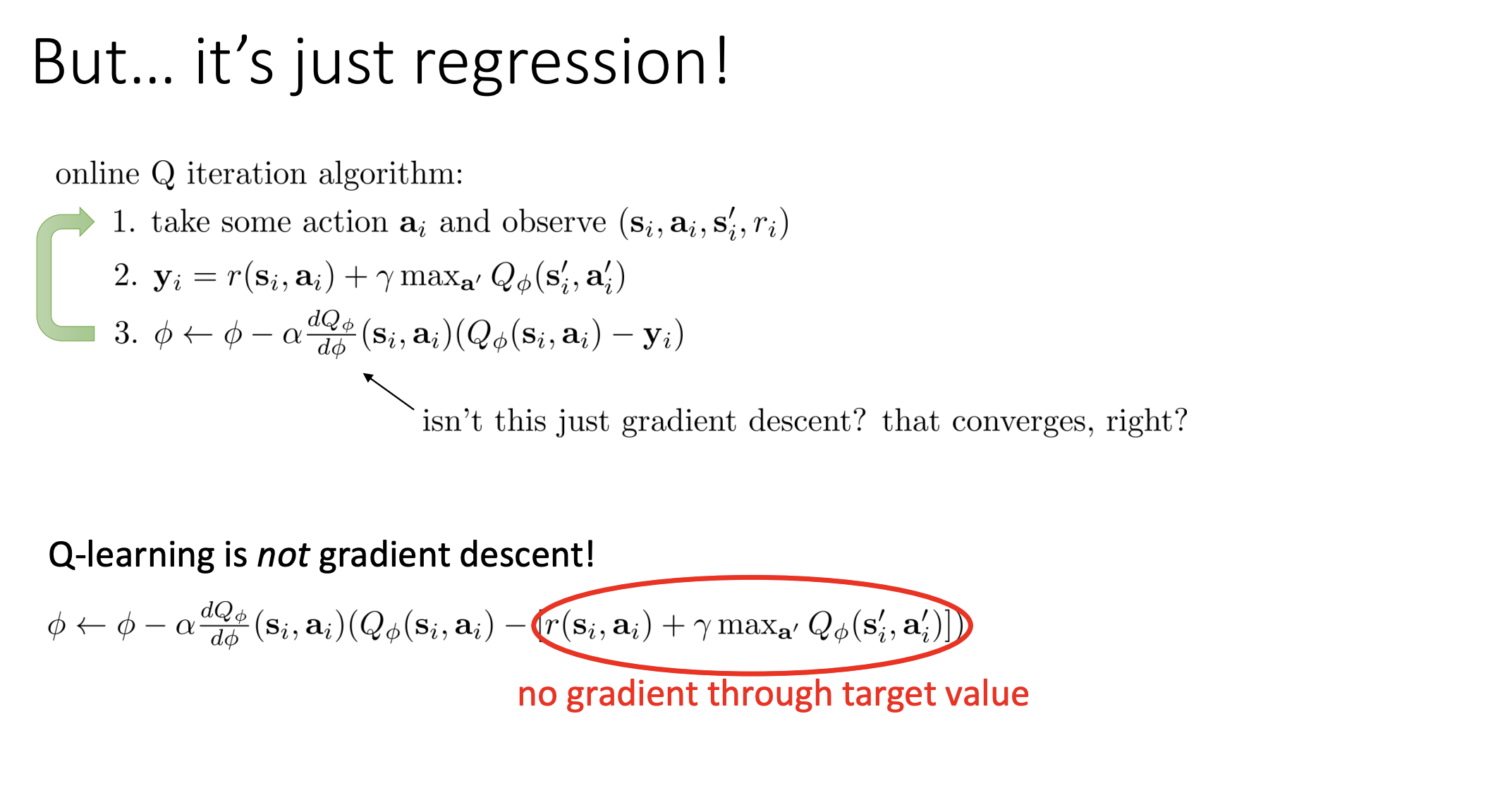
Online Q-learning algorithms

Online Q-iteration algorithm:

1. take some action $\mathbf{a}_i$ and observe $(\mathbf{s}_i,\mathbf{a}_i,\mathbf{s}_i^\prime,r_i)$
2. $\mathbf{y}_i=r(\mathbf{s}_i,\mathbf{a}_i)+\gamma\max_{\mathbf{a}^{\prime}}Q_\phi(\mathbf{s}_i^{\prime},\mathbf{a}_i^{\prime})$
3. $\phi\leftarrow\phi-\alpha\frac{dQ_\phi}{d\phi}(\mathbf{s}_i,\mathbf{a}_i)(Q_\phi(\mathbf{s}_i,\mathbf{a}_i)-\mathbf{y}_i)$

This is the basic online Q-learning algorithm, also sometimes called Watkins Q-learning. But actually the observation part is off-policy. There’s no need to take actions using the latest greedy policy.

So what policy should we use? The final policy will be the greedy policy. If Q-learning converges and has error equals to zero, then we know the greedy policy is the optimal policy. But while learning is progressing, using the greedy policy may not be such a good idea.

Part of reason why we might not want to do this is that this $\arg \max$ policy is deterministic and if the initial Q-function is quite bad, it’s not going to be random, but it’s going to be arbitrary, then it will essentially commit the $\arg \max$ policy take the same action every time it enters a particular state. And if that action is not a very good action, we might be stuck taking that bad action essentially in perpetuity and we might never discover that better actions exist.

So in practice, when we run fitted Q-learning algorithms, it’s highly desirable to modify the policy that we use in Step 1 to not just be the $\arg \max$ policy, but to inject some additional randomness to produce better exploration.

There’re number of choices that we make in practice to facilitate this.

• Epsilon greedy

  

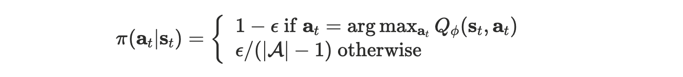
  With probability $1 - \epsilon$ , we will take the greedy action and then with probability $\epsilon$ , we will take one of the other actions uniformly at random.

• Boltzmann exploration / Softmax exploration

  $$ \pi(\mathbf{a}_t|\mathbf{s}_t)\propto\exp(Q_\phi(\mathbf{s}_t,\mathbf{a}_t)) $$

  Select the actions in proportion to some positive transformation of the Q-values. A particularly popular positive transformation is exponentiation. In this case, the best actions will be the most frequent. The actions that are almost as good as the best action will also be quite frequent because they’ll have similarly high probabilities.

  This method can be more preferred than the epsilon greedy because if there are two actions that are about equally good, we’ll take them about an equal number of times. And also for those bad action already known, we don’t want to waste time exploring it.

Value Functions in Theory

Value function learning theory

Let’s start with the value iteration algorithm:

1. set $Q(\mathbf{s}, \mathbf{a}) \leftarrow r(\mathbf{s},\mathbf{a}) + \gamma E[V(\mathbf{s}^\prime)]$
2. set $V(\mathbf{s}) \leftarrow \max_\mathbf{a}Q(\mathbf{s}, \mathbf{a})$

Dose it converge? And if so, to what?

Define an operator $\mathcal{B}$, which is known as the Bellman Operator. The Bellman Operator, when applied to a value function ( when the value function is a table, it’s just a vector of numbers ), it performs the following operation

$$ \mathcal{B}V = \max_{\mathbf{a}}(r_{\mathbf{a}} + \gamma\mathcal{T}_{\mathbf{a}}V) $$

where $\mathcal{T}_{\mathbf{a}}$ is a matrix in which every entry is the probability of $p(\mathbf{s}^\prime | \mathbf{s}, \mathbf{a})$, so basically it’s computing the expectation as a linear operator.

• $r_{\mathbf{a}}$: stacked vector of rewards at all states for action $\mathbf{a}$
• $\mathcal{T}_\mathbf{a}$: matrix of transitions for action $\mathbf{a}$ such that $\mathcal{T}_{\mathbf{a}, i, j} = p(\mathbf{s}^\prime = i | \mathbf{s} = j, \mathbf{a})$

So this representation captures the value iteration algorithm.

$V^ \star$ is a fixed point of $\mathcal{B}$, where

$$ \begin{aligned}V^\star(\mathbf{s})=\max_\mathbf{a}r(\mathbf{s},\mathbf{a})+\gamma E[V^\star(\mathbf{s^{\prime}})]\end{aligned} $$

which means that $V^{\star}=\mathcal{B}V^{\star}$. What’s more, $V^\star$ is the optimal value function and if we use the $\arg \max$ policy with respect to that, we’ll get the optimal policy. It actually can be proved that the fixed point always exits, is always unique and always corresponds to the optimal policy. The only problem is, does repeatedly applying $\mathcal{B}$ to $V$ always reach this fixed point.

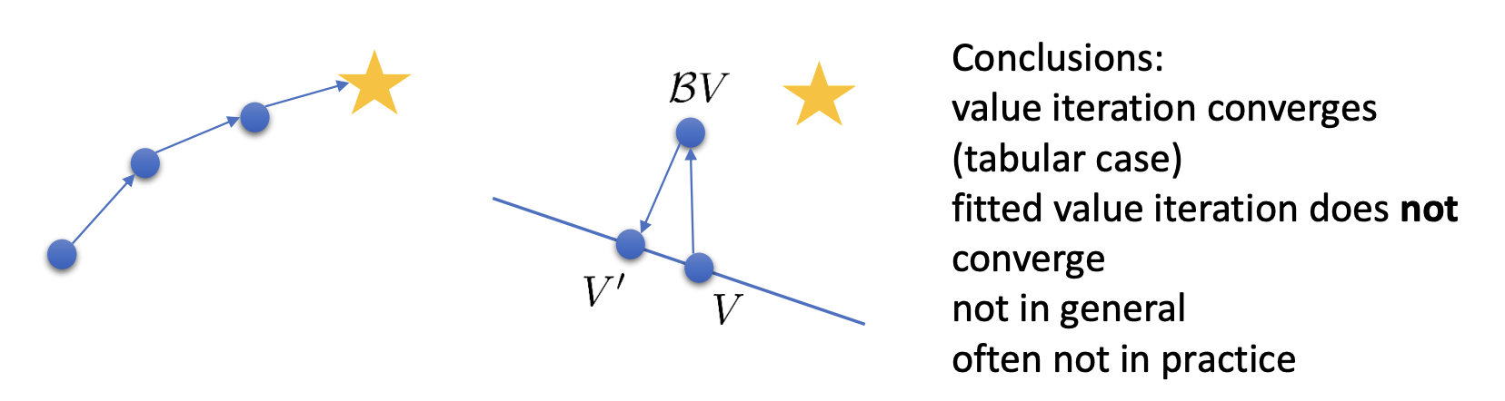
We can prove that value iteration reaches $V^\star$ because $\mathcal{B}$ is a contraction.

• contraction: for any $V$ and $\bar{V}$ , we have $|\mathcal{B}V-\mathcal{B}\bar{V}|_\infin\leq\gamma|V-\bar{V}|_\infin$

Up till now, the value iteration algorithm can be written extremely concisely as just repeatedly applying only one step:

1. $V\leftarrow\mathcal{B}V$

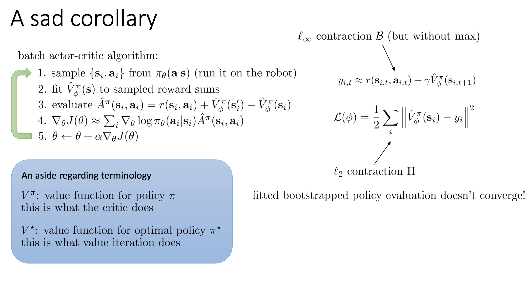
Non-tabular value function learning

Now let’s go to the fitted value iteration algorithm. Different from the value iteration algorithm, the fitted value iteration algorithm is has a extra Step 2 which trains the neural network.

1. set $\phi\leftarrow\arg\min_\phi\frac{1}{2}\sum_i\left|V_\phi(\mathbf{s}_i)-\mathbf{y}_i\right|^2$

Abstractly, one of the ways we can think the supervised learning is that we have some set of value functions that we can represent. That set, if the value functions are neural network, are actually continuous that consists of all possible neural nets with particular architecture, but with different weight values. We’ll denote that set as a set $\Omega$ and in supervised learning we sometimes refer to this as the hypothesis set or the hypothesis space. Supervised learning consists of finding an element in the hypothesis space that optimize the objective, which is the squared difference between $V_{\phi}(\mathbf{s}_i)$ and the target value $\mathbf{y}_i$ . The target value is basically $\mathcal{B}V$ concluded in Step 1.

So the entire fitted value iteration algorithm can be seen as repeatedly finding a new value function $V^\prime$ which is the $\arg \min$ inside the set $\Omega$ of the squared difference between $V^{\prime}$ and $\mathcal{B}V$.

$$ V^{\prime}\leftarrow\arg\min_{V^{\prime}\in\Omega}\frac{1}{2}\sum|V^{\prime}(\mathbf{s})-(\mathcal{B}V)(\mathbf{s})|^2 $$

• $\Omega$: all value functions represented by, e.g., neural nets
• $(\mathcal{B}V)(\mathbf{s})$: updated value function

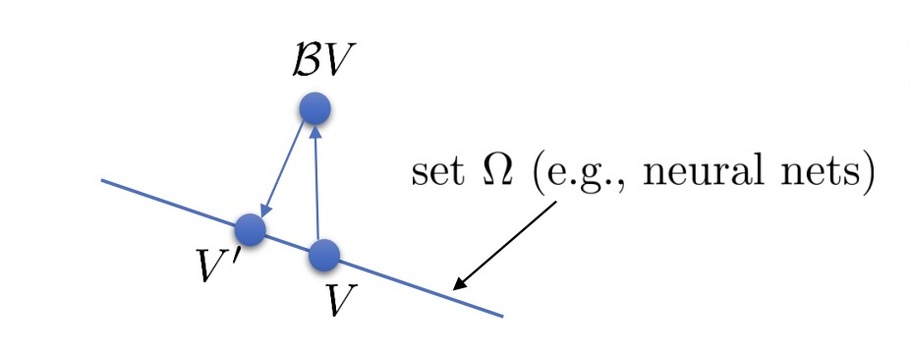
This can be seen, vividly, as a projection. We denote this new operator of projection as $\Pi$, where

$$ \begin{aligned}\Pi V=\arg\min_{V^{\prime}\in\Omega}\frac{1}{2}\sum|V^{\prime}(\mathbf{s})-V(\mathbf{s})|^2\end{aligned} $$

Again, the fitted value iteration algorithm can be written extremely concisely as

1. $V \leftarrow \Pi \mathcal{B}V$

• $\mathcal{B}$ is a contraction w.r.t. $\infin$-norm ( “max” norm ), $|\mathcal{B}V-\mathcal{B}\bar{V}|_{\infin}\leq\gamma|V-\bar{V}|_{\infin}$
• $\Pi$ is a contraction w.r.t. $l_2$-norm ( Euclidean distance ), $|\Pi V-\Pi\bar{V}|^2\leq|V-\bar{V}|^2$

BUT… $\Pi \mathcal{B}$ is not a contraction of any kind, because they are contractions for different norms. The picture describes it vividly.

What about fitted Q-iteration?

Fitted Q-iteration algorithm:

1. set $\mathbf{y}_i\leftarrow r(\mathbf{s}_i,\mathbf{a}_i)+\gamma E[V _\phi(\mathbf{s}_i^{\prime})]$
2. set $\phi\leftarrow\arg\min_\phi\frac{1}{2}\sum_i\left|Q_\phi(\mathbf{s}_i,\mathbf{a}_i)-\mathbf{y}_i\right|^2$

We can do the similar things

• define an operator $\mathcal{B}$ : $\mathcal{B}Q = r + \gamma \mathcal{T} \max_{\mathbf{a}}Q$ ( $\max$ now after the transition operator )
• define an operator $\Pi$ : $\Pi Q = \arg \min_{Q^\prime \in \Omega} \frac{1}{2} \sum | Q^\prime (\mathbf{s} , \mathbf{a}) - Q(\mathbf{s}, \mathbf{a}) |^2$

So the concise version is:

1. $Q \leftarrow \Pi \mathcal{B}Q$

Also, $\Pi \mathcal{B}$ is not a contraction of any kind.