Lecture 9: Advanced Policy Gradient

Lecture Slides & Videos

Why does the policy gradient work?

Conceptually, we can think of a more general way of looking at policy gradient.

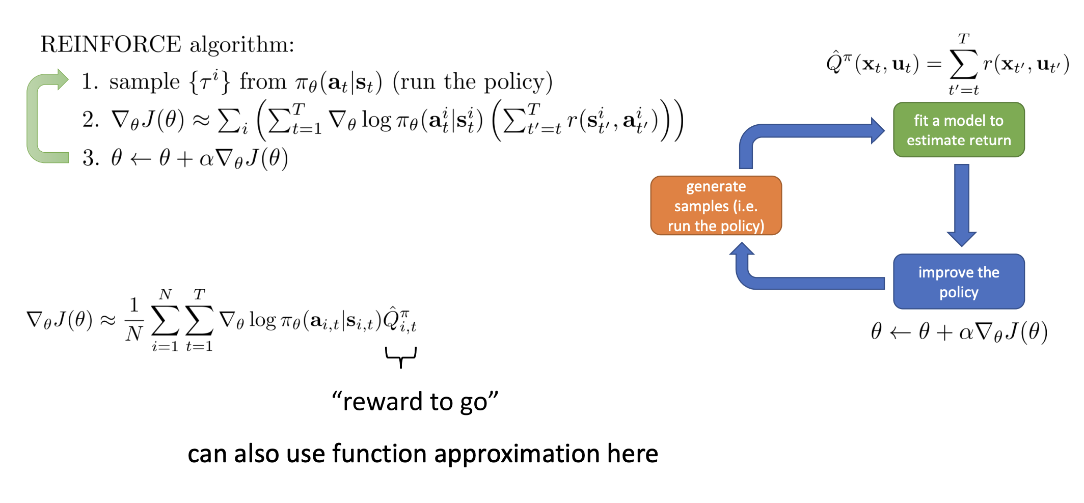
Estimate $\hat{A}^{\pi}(\mathbf{s}_t, \mathbf{a}_t)$ for current policy $\pi$
Use $\hat{A}^{\pi}(\mathbf{s}_t, \mathbf{a}_t)$ to get improved policy $\pi^{\prime}$

This way of looking at the policy gradient is basically equivalent to the Recap, where we estimate $\hat{A}$ by generating samples and summing up the reward-to-go and then use $\hat{A}$ to improve the policy by calculating the policy gradient and doing a step of gradient descent. What we’re really doing is, in some extent, alternating these two steps.

It is quite apparent that the policy gradient are very related to the policy iteration algorithm.

Evaluate $A^\pi(\mathbf{s}, \mathbf{a})$
set $\pi \leftarrow \pi^\prime$

In both cases, we alternate between estimating the value of the current policy and then using the estimated value to improve that policy.

One of the main differences is that in the policy iteration, when we calculate the new policy $\pi^\prime$, we use the $\arg \max$ rule, picking the policy $\pi^\prime$ that assigns the a probability of $1$ to the action that is $\arg \max$ of the current advantages. In the policy gradient, however, we make a much gentler update. It doesn’t immediately jump to $\arg \max$ , but improves a little bit in the direction where the advantages are large. So the policy gradient can somehow be seen as a softened version of the policy iteration procedure.

Policy gradient as policy iteration

We use $J(\theta)$ to represent the reinforcement learning objective.

$$ J(\theta)=E_{\tau\sim p_{\theta}(\tau)}\left[\sum_t\gamma^tr(\mathbf{s}_t,\mathbf{a}_t)\right] $$

Claim

$$ J(\theta^{\prime})-J(\theta)=E_{\tau\sim p_{\theta^{\prime}}(\tau)}\left[\sum_{t}\gamma^{t}A^{\pi_{\theta}}(\mathbf{s}_{t},\mathbf{a}_{t})\right] $$

Let’s unpack this statement to try to get some intuition for why we even want to care about this.

$J(\theta^{\prime})-J(\theta)$: The improvement in the RL objective that we get from going from the old parameter $\theta$ to the new parameter $\theta^\prime$.
- $\max_{\theta^\prime}{ J(\theta^\prime) } \iff \max_{\theta^{\prime}} { J(\theta^{\prime}) - J(\theta) } \iff \max_{\theta^\prime} { E_{\tau\sim p_{\theta^{\prime}}(\tau)}\left[\sum_{t}\gamma^{t}A^{\pi_{\theta}}(\mathbf{s}_{t},\mathbf{a}_{t})\right] }$
The right hand side is expressing the expected value under the trajectory distribution induced by the new policy of the advantage of the old policy.
- $\iff$Policy iteration computes the advantage of the old policy $A^{\pi_{\theta}}$ and then uses that advantage to find a new improved policy by $\theta^\prime$.

If the claim can be proven, then we can show that using the advantage of the old policy and maximizing under the new policy is a correct way to optimize the new policy.

Prove

$$ \begin{aligned}J(\theta^{\prime})-J(\theta) & =J(\theta^{\prime})-E_{\mathbf{s}_0\sim p(\mathbf{s}_0)}\left[V^{\pi_\theta}(\mathbf{s}_0)\right] \\ & =J(\theta^{\prime})-E_{\tau\sim p_{\theta^{\prime}}(\tau)}\left[V^{\pi_\theta}(\mathbf{s}_0)\right] \\ & =J(\theta^{\prime})-E_{\tau\sim p_{\theta^{\prime}}(\tau)}\left[\sum_{t=0}^\infty\gamma^tV^{\pi_\theta}(\mathbf{s}_t)-\sum_{t=1}^\infty\gamma^tV^{\pi_\theta}(\mathbf{s}_t)\right] \\ & =J(\theta^{\prime})+E_{\tau\sim p_{\theta^{\prime}}(\tau)}\left[\sum_{t=0}^\infty\gamma^t(\gamma V^{\pi_\theta}(\mathbf{s}_{t+1})-V^{\pi_\theta}(\mathbf{s}_t))\right] \\ & =E_{\tau\sim p_{\theta^{\prime}}(\tau)}\left[\sum_{t=0}^\infty\gamma^tr(\mathbf{s}_t,\mathbf{a}_t)\right]+E_{\tau\sim p_{\theta^{\prime}}(\tau)}\left[\sum_{t=0}^\infty\gamma^t(\gamma V^{\pi_\theta}(\mathbf{s}_{t+1})-V^{\pi_\theta}(\mathbf{s}_t))\right] \\ & =E_{\tau\sim p_{\theta^{\prime}}(\tau)}\left[\sum_{t=0}^\infty\gamma^t(r(\mathbf{s}_t,\mathbf{a}_t)+\gamma V^{\pi_\theta}(\mathbf{s}_{t+1})-V^{\pi_\theta}(\mathbf{s}_t))\right] \\ & =E_{\tau\sim p_{\theta^{\prime}}(\tau)}\left[\sum_{t=0}^\infty\gamma^tA^{\pi_\theta}(\mathbf{s}_t,\mathbf{a}_t)\right] \end{aligned} $$

So now the RL objective has changed into maximizing

$$ E_{\tau\sim p_{\theta^{\prime}}(\tau)}\left[\sum_{t}\gamma^{t}A^{\pi_{\theta}}(\mathbf{s}_{t},\mathbf{a}_{t})\right] $$

expectation under $\pi_{\theta^\prime}$
advantage under $\pi_\theta$

This can be written out as

$$ E_{\tau\sim p_{\theta^{\prime}}(\tau)}\left[\sum_t\gamma^tA^{\pi_\theta}(\mathbf{s}_t,\mathbf{a}_t)\right]=\sum_tE_{\mathbf{s}_t\sim p_{\theta^{\prime}}(\mathbf{s}_t)}\left[E_{\mathbf{a}_t\sim\pi_{\theta^{\prime}}(\mathbf{a}_t|\mathbf{s}_t)}\left[\gamma^tA^{\pi_\theta}(\mathbf{s}_t,\mathbf{a}_t)\right]\right] $$

At this point, if we wanted to actually write down a policy gradient procedure for optimizing this objective, we could recall the Importance Sampling mentioned in Lecture 5.

$$ \begin{aligned}E_{x\thicksim p(x)}[f(x)] & =\int p(x)f(x)dx \\ & \begin{aligned}=\int\frac{q(x)}{q(x)}p(x)f(x)dx\end{aligned} \\ & =\int q(x)\frac{p(x)}{q(x)}f(x)dx \\ & =E_{x\thicksim q(x)}\left[\frac{p(x)}{q(x)}f(x)\right]\end{aligned} $$

$$ E_{\tau\sim p_{\theta^{\prime}}(\tau)}\left[\sum_t\gamma^tA^{\pi_\theta}(\mathbf{s}_t,\mathbf{a}_t)\right]= \sum_tE_{\mathbf{s}_t\sim p_{\theta^{\prime}}(\mathbf{s}_t)}\left[E_{\mathbf{a}_t\sim\pi_\theta(\mathbf{a}_t|\mathbf{s}_t)}\left[\frac{\pi_{\theta^{\prime}}(\mathbf{a}_t|\mathbf{s}_t)}{\pi_\theta(\mathbf{a}_t|\mathbf{s}_t)}\gamma^tA^{\pi_\theta}(\mathbf{s}_t,\mathbf{a}_t)\right]\right] $$

As mentioned in Lecture 5, we could get policy gradient just by differentiating an equation very similar. The only difference is that the states are still distributed according to $p_{\theta^\prime}$, instead of $p_\theta$.

We can’t sample from $p_{\theta^\prime}(\mathbf{s}_t)$ because we don’t yet know what the $\theta^\prime$ will be. Is it OK to use $p_{\theta}(\mathbf{s}_t)$ instead?

Ignoring distribution mismatch?

Essentially, we need to somehow ignore the fact that we need to use states sampled from $p_{\theta^\prime}(\mathbf{s}_t)$ and instead using $p_{\theta}(\mathbf{s}_t)$ , which means that we need following statement to be true

$$ \sum_{t}E_{\mathbf{s}_{t}\sim p_{\theta^{\prime}}(\mathbf{s}_{t})}\left[E_{\mathbf{a}_{t}\sim\pi_{\theta}(\mathbf{a}_{t}|\mathbf{s}_{t})}\left[\frac{\pi_{\theta^{\prime}}(\mathbf{a}_{t}|\mathbf{s}_{t})}{\pi_{\theta}(\mathbf{a}_{t}|\mathbf{s}_{t})}\gamma^{t}A^{\pi_{\theta}}(\mathbf{s}_{t},\mathbf{a}_{t})\right]\right]\approx\sum_{t}E_{\mathbf{s}_{t}\sim p_{\theta}(\mathbf{s}_{t})}\left[E_{\mathbf{a}_{t}\sim\pi_{\theta}(\mathbf{a}_{t}|\mathbf{s}_{t})}\left[\frac{\pi_{\theta^{\prime}}(\mathbf{a}_{t}|\mathbf{s}_{t})}{\pi_{\theta}(\mathbf{a}_{t}|\mathbf{s}_{t})}\gamma^{t}A^{\pi_{\theta}}(\mathbf{s}_{t},\mathbf{a}_{t})\right]\right] $$

Claim: $p_{\theta}(\mathbf{s}_t)$ is close to $p_{\theta^\prime}(\mathbf{s}_t)$ when $\pi_\theta$ is close to $\pi_{\theta^\prime}$.

Let

$$ \bar{A}(\theta^\prime) = \sum_{t}E_{\mathbf{s}_{t}\sim p_{\theta}(\mathbf{s}_{t})}\left[E_{\mathbf{a}_{t}\sim\pi_{\theta}(\mathbf{a}_{t}|\mathbf{s}_{t})}\left[\frac{\pi_{\theta^{\prime}}(\mathbf{a}_{t}|\mathbf{s}_{t})}{\pi_{\theta}(\mathbf{a}_{t}|\mathbf{s}_{t})}\gamma^{t}A^{\pi_{\theta}}(\mathbf{s}_{t},\mathbf{a}_{t})\right]\right] $$

This surrogate objective fully depends on $p_{\theta}$. So the training data is generated on the old policy $\pi_\theta$. The optimization procedure is fully off-line.

$$ J(\theta^{\prime})-J(\theta)\approx\bar{A}(\theta^{\prime})\quad\Rightarrow\quad\theta^{\prime}\leftarrow\arg\max_{\theta^{\prime}}\bar{A}(\theta) $$

This allows us to do Step 2: Use $\hat{A}^\pi(\mathbf{s}_t,\mathbf{a}_t)$ to get improved policy $\pi^\prime$.

Bounding the Distribution Change

Simple case

Assume $\pi_{\theta}$ is a deterministic policy $\mathbf{a}_t = \pi_{\theta}(\mathbf{s}_t)$.

$\pi_{\theta^{\prime}}$ is close to $\pi_{\theta}$ if $\pi_{\theta^{\prime}}(\mathbf{a}_t\neq\pi_\theta(\mathbf{s}_t)|\mathbf{s}_t)\leq\epsilon$

In this case, we can write the state marginal as

$$ p_{\theta^{\prime}}(\mathbf{s}_{t})=(1-\epsilon)^tp_\theta(\mathbf{s}_t)+(1-(1-\epsilon)^t))p_{\mathrm{mistake}}(\mathbf{s}_t) $$

$(1-\epsilon)^t$: the probability we make no mistakes
$p_{\mathrm{mistake}}(\mathbf{s}_t)$: some other distribution
- Assume that we know nothing about it, e.g., it could be a tightrope walker from the imitation learning.

This implies that we can write the total variation divergence between $p_{\theta^{\prime}}$ and $p_{\theta}$ as

$$ |p_{\theta^{\prime}}(\mathbf{s}_t)-p_\theta(\mathbf{s}_t)|=(1-(1-\epsilon)^t)|p_\mathrm{mistake}(\mathbf{s}_t)-p_\theta(\mathbf{s}_t)| \leq2(1-(1-\epsilon)^t) $$

Given that $(1-\epsilon)^t\geq1-\epsilon t \space \text{for} \space \epsilon\in [0, 1]$, we are able to express the bound as a quantity that is linear in $\epsilon$ and $t$

$$ |p_{\theta^{\prime}}(\mathbf{s}_t)-p_\theta(\mathbf{s}_t)| \leq2\epsilon t $$

Basically, this analysis was once mentioned in Lecture 2.

General case

$\pi_{\theta^\prime}$ is close to $\pi_\theta$ if $|\pi_{\theta^{\prime}}(\mathbf{a}_t|\mathbf{s}_t)-\pi_\theta(\mathbf{a}_t|\mathbf{s}_t)|\leq\epsilon$ for all $\mathbf{s}_t$
- This will also hold true if the boundless point is in expectation, meaning that the expected value of the total variation divergence ( TVD ) is less than or equal to $\epsilon$.

We will use a useful lemma: if $|p_X(x)-p_Y(x)|=\epsilon$, exists $p(x, y)$ such that $p(x) = p_X(x)$ and $p(y) = p_Y(y)$ and $p(x=y) = 1 - \epsilon$.

$\Rightarrow$ Essentially this says that $p_X(x)$ “agrees” with $p_Y(y)$ with probability $\epsilon$

$\Rightarrow$ $\pi_{\theta^\prime}(\mathbf{a}_t | \mathbf{s}_t)$ takes a different action than $\pi_{\theta}(\mathbf{a}_t | \mathbf{s}_t)$ with probability at most $\epsilon$

This lemma allows us to state the same result that we had in the simple case.

$$ |p_{\theta^{\prime}}(\mathbf{s}_t)-p_\theta(\mathbf{s}_t)|=(1-(1-\epsilon)^t)|p_\mathrm{mistake}(\mathbf{s}_t)-p_\theta(\mathbf{s}_t)|\leq2\epsilon t $$

Above is the result that we have on the state marginals.

Then we’re going to derive another calculation which describes the expected value of functions under distributions when the total variation divergence between those distributions is bounded. We have

$$ \begin{aligned} \begin{aligned} E_{p_{\theta^{\prime}}(\mathbf{s}_t)}[f(\mathbf{s}_t)]=\sum_{\mathbf{s}_t}p_{\theta^{\prime}}(\mathbf{s}_t)f(\mathbf{s}_t) \end{aligned} & \begin{aligned} \geq\sum_{\mathbf{s}_t}p_\theta(\mathbf{s}_t)f(\mathbf{s}_t)-|p_\theta(\mathbf{s}_t)-p_{\theta^{\prime}}(\mathbf{s}_t)|\max_{\mathbf{s}_t}f(\mathbf{s}_t) \end{aligned} \\ & \geq E_{p_\theta(\mathbf{s}_t)}[f(\mathbf{s}_t)]-2\epsilon t\max_{\mathbf{s}_t}f(\mathbf{s}_t) \end{aligned} $$

So when we go back to the original statement, we have arrived at

$$ \sum_tE_{\mathbf{s}_t\sim p_{\theta^{\prime}}(\mathbf{s}_t)}\left[E_{\mathbf{a}_t\sim\pi_\theta(\mathbf{a}_t|\mathbf{s}_t)}\left[\frac{\pi_{\theta^{\prime}}(\mathbf{a}_t|\mathbf{s}_t)}{\pi_\theta(\mathbf{a}_t|\mathbf{s}_t)}\gamma^tA^{\pi_\theta}\left(\mathbf{s}_t,\mathbf{a}_t\right)\right]\right]\geq \sum_tE_{\mathbf{s}_t\sim p_\theta(\mathbf{s}_t)}\left[E_{\mathbf{a}_t\sim\pi_\theta(\mathbf{a}_t|\mathbf{s}_t)}\left[\frac{\pi_{\theta^{\prime}}(\mathbf{a}_t|\mathbf{s}_t)}{\pi_\theta(\mathbf{a}_t|\mathbf{s}_t)}\gamma^tA^{\pi_\theta}\left(\mathbf{s}_t,\mathbf{a}_t\right)\right]\right]-\sum_t2\epsilon tC $$

where the constant $C$ is the largest value that the thing inside the state expectation can take on. In fact, the quantity inside the bracket is basically some expected value of an advantage, which is the sum of the sum of rewards over time. Therefore, $C$ should be $O(Tr_{\text{max}})$ or, if taking a discount $\gamma$, $O(\frac{r_{\text{max}}}{1 - \gamma})$.

To sum up a little bit, what we have so far basically shows that as long as $\pi_{\theta^\prime}$ is close enough to $\pi_{\theta}$

$$ |\pi_{\theta^{\prime}}(\mathbf{a}_t|\mathbf{s}_t)-\pi_\theta(\mathbf{a}_t|\mathbf{s}_t)|\leq\epsilon $$

it is a good way to maximize the RL objective through

$$ \theta^{\prime}\leftarrow\arg\max_{\theta^{\prime}}\sum_{t}E_{\mathbf{s}_{t}\sim p_{\theta}(\mathbf{s}_{t})}\left[E_{\mathbf{a}_{t}\sim\pi_{\theta}(\mathbf{a}_{t}|\mathbf{s}_{t})}\left[\frac{\pi_{\theta^{\prime}}(\mathbf{a}_{t}|\mathbf{s}_{t})}{\pi_{\theta}(\mathbf{a}_{t}|\mathbf{s}_{t})}\gamma^{t}A^{\pi_{\theta}}(\mathbf{s}_{t},\mathbf{a}_{t})\right]\right] $$

because for small enough $\epsilon$, this is guaranteed to improve $J(\theta^{\prime})-J(\theta)$.

Policy Gradients with Constraints

A more convenient bound

Actually the total variation divergence is also bounded

$$ \begin{aligned}|\pi_{\theta^{\prime}}(\mathbf{a}_t|\mathbf{s}_t)-\pi_\theta(\mathbf{a}_t|\mathbf{s}_t)|\leq\sqrt{\frac{1}{2}D_{\mathrm{KL}}(\pi_{\theta^{\prime}}(\mathbf{a}_t|\mathbf{s}_t)|\pi_\theta(\mathbf{a}_t|\mathbf{s}_t))}\end{aligned} $$

$\Rightarrow$ $D_{\mathrm{KL}}(\pi_{\theta^{\prime}}(\mathbf{a}_t|\mathbf{s}_t)|\pi_\theta(\mathbf{a}_t|\mathbf{s}_t))$ bounds state marginal difference

Therefore, KL divergence will be a more convenient bound.

$$ D_{\mathrm{KL}}(p_1(x)|p_2(x))=E_{x\sim p_1(x)}\left[\log\frac{p_1(x)}{p_2(x)}\right] $$

It’s basically the most widely used type of divergence measure between distributions. It can be very convenient because it has tractable expressions expressed expected value of $\log$ probabilities and many continuous value distributions have tractable closed form solutions for the KL divergence.

The KL divergence is differentiable so long as the two distributions have the same support. That why for the convenience, we will express the constraint as a KL divergence rather than a total variation divergence, and since the KL divergence bounds the total variation divergence, this is a legitimate thing to do.

So in practice, the “close” bound would be

$$ D_{\mathrm{KL}}(\pi_{\theta^{\prime}}(\mathbf{a}_t|\mathbf{s}_t)|\pi_\theta(\mathbf{a}_t|\mathbf{s}_t))\leq\epsilon $$

How do we enforce the constraint?

There are a number of different method to enforce the constraint. A very simple one is to write out an objective in terms of the Lagrangian of this constrained optimization.

$$ \mathcal{L}(\theta^{\prime},\lambda)=\sum_{t}E_{\mathbf{s}_{t}\sim p_{\theta}(\mathbf{s}_{t})}\left[E_{\mathbf{a}_{t}\sim\pi_{\theta}(\mathbf{a}_{t}|\mathbf{s}_{t})}\left[\frac{\pi_{\theta^{\prime}}(\mathbf{a}_{t}|\mathbf{s}_{t})}{\pi_{\theta}(\mathbf{a}_{t}|\mathbf{s}_{t})}\gamma^{t}A^{\pi_{\theta}}(\mathbf{s}_{t},\mathbf{a}_{t})\right]\right]-\lambda(D_{\mathrm{KL}}(\pi_{\theta^{\prime}}(\mathbf{a}_{t}|\mathbf{s}_{t})|\pi_{\theta}(\mathbf{a}_{t}|\mathbf{s}_{t}))-\epsilon) $$

One of the things we can do to solve a constrained optimization problem is to alternate between maximizing the Lagrangian with respect of the primal variable, $\theta^\prime$ , and then taking a gradient descent step on the dual variables.

Maximize $\mathcal{L}(\theta^{\prime},\lambda)$ with respect to $\theta^\prime$ ( can do this incompletely, for only a few grad steps )
$\lambda\leftarrow\lambda+\alpha(D_{\mathrm{KL}}(\pi_{\theta^{\prime}}(\mathbf{a}_t|\mathbf{s}_t)|\pi_\theta(\mathbf{a}_t|\mathbf{s}_t))-\epsilon)$

The intuition is raising $\lambda$ if constraint is violated too much, else lowering it. This is actually an instance of dual gradient descent ( more on this later ).

Natural Gradient

Basically the objective is

When we calculate the gradient of some objective and we use gradient ascent or gradient descent, that can be interpreted as optimizing a first-order Taylor expansion of that objective.

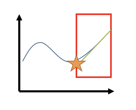
For example, if we want to optimize some complicated function like the blue curve here, one way we can do is that we can pick up a region and compute a very simple approximation, e.g., linear approximation, to that function ( green line here, basically obtained by taking the gradient ). Then, instead of optimizing the blue curve, we optimize the green line, which is much simpler than the blue curve.

But if we don’t impose any constraint, the green line goes to positive and negative infinity. So this only makes sense if we impose a constraint, which is essentially the region ( red box here ) within which we trust the degree to which the green line approximates the blue curve.

If we are minimizing, then we would pick the point on the edge of the red region where the green function has the lowest value, which will hopefully also be a point ( star point ) where the blue function has a lower value.

We can change our optimization objective into

$$ \theta^\prime \leftarrow \arg \max_{\theta^\prime} \nabla_\theta \bar{A}(\theta)^T (\theta^\prime - \theta) $$

This process of using first order Taylor approximation for objective is also known as linearization.

One really appealing thing about simplifying in this way is that $\nabla_\theta \bar{A}(\theta)$ is going to be exactly the normal policy gradient ( derivation mentioned in Lecture 5 ).

$$ \nabla_{\theta^{\prime}}\bar{A}(\theta^{\prime})=\sum_{t}E_{\mathbf{s}_{t}\sim p_{\theta}(\mathbf{s}_{t})}\left[E_{\mathbf{a}_{t}\sim\pi_{\theta}(\mathbf{a}_{t}|\mathbf{s}_{t})}\left[\frac{\pi_{\theta^{\prime}}(\mathbf{a}_{t}|\mathbf{s}_{t})}{\pi_{\theta}(\mathbf{a}_{t}|\mathbf{s}_{t})}\gamma^{t}\nabla_{\theta^{\prime}}\log\pi_{\theta^{\prime}}(\mathbf{a}_{t}|\mathbf{s}_{t})A^{\pi_{\theta}}(\mathbf{s}_{t},\mathbf{a}_{t})\right]\right] \\ \nabla_{\theta}\bar{A}(\theta)=\sum_{t}E_{\mathbf{s}_{t}\sim p_{\theta}(\mathbf{s}_{t})}\left[E_{\mathbf{a}_{t}\sim\pi_{\theta}(\mathbf{a}_{t}|\mathbf{s}_{t})}\left[\frac{\pi_{\theta}(\mathbf{a}_{t}|\mathbf{s}_{t})}{\pi_{\theta}(\mathbf{a}_{t}|\mathbf{s}_{t})}\gamma^{t}\nabla_{\theta}\log\pi_{\theta}(\mathbf{a}_{t}|\mathbf{s}_{t})A^{\pi_{\theta}}(\mathbf{s}_{t},\mathbf{a}_{t})\right]\right] \\ \nabla_\theta\bar{A}(\theta)=\sum_tE_{\mathbf{s}_t\sim p_\theta(\mathbf{s}_t)}\left[E_{\mathbf{a}_t\sim\pi_\theta(\mathbf{a}_t|\mathbf{s}_t)}\left[\gamma^t\nabla_\theta\log\pi_\theta(\mathbf{a}_t|\mathbf{s}_t)A^{\pi_\theta}(\mathbf{s}_t,\mathbf{a}_t)\right]\right]=\nabla_\theta J(\theta) $$

Can we just use the gradient then?

Now we have derived

$$ \theta^{\prime}\leftarrow\arg\max_{\theta^{\prime}}\nabla_\theta J(\theta)^T(\theta^{\prime}-\theta) $$

Can we just use the gradient descent/ascent then? If we just calculating the policy gradient, the process will be

$$ \theta\leftarrow\theta+\alpha\nabla_\theta J(\theta) $$

The problem with doing this is that, as we change $\theta$ , the probabilities of the new policy $\pi_{\theta} (\mathbf{a}_t | \mathbf{s}_t)$ will change by different amount because some parameters ( some entries in $\theta$ ) affect the probabilities more than others. So in general, taking a step like this will usually not respect the KL divergence constraint because there might have some very small changes in a parameter but that parameter might have a very large influence on the probabilities.

The gradient descent/ascent actually solves this constrained optimization problem.

$$ \theta^{\prime}\leftarrow\arg\max_{\theta^{\prime}}\nabla_\theta J(\theta)^T(\theta^{\prime}-\theta) $$

such that $|\theta-\theta^{\prime}|^2\leq\epsilon$.

This only guarantees the parameters to be “close”, rather than the policies.

What’s more, the largest length of that gradient step will be constrained by $\epsilon$. In fact, the learning rate in gradient descent/ascent can actually be obtained as the Lagrange multiplier for this constraint and a close form equation can be derived for it.

$$ \theta^{\prime}=\theta+\sqrt{\frac{\epsilon}{|\nabla_\theta J(\theta)|^2}}\nabla_\theta J(\theta) $$

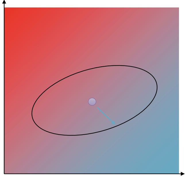
The gradient descent/ascent does actually solve a constrained optimization problem, but it’s the wrong constraint. The constraint is in the $\theta$ space instead of the distribution space. Intuitively, the constraint shape is a circle for gradient descent, but we want it to be a kind of ellipse. We want the ellipse to be squished along the highly sensitive direction, a tighter constraint in the direction of $\theta$ that results in big changes in probability. We want the ellipse to be elongated in the directions of where large changes in $\theta$ result in small changes in probability.

The way we’re going to do this is by doing the same thing to the constraint that we did to the objective.

For the constraint, we use a second-order Taylor expansion around the point $\theta^\prime = \theta$. We don’t use a first-order Taylor expansion because the KL divergence has a derivative of $0$ at $\theta^\prime = \theta$, but the second derivative is not.

$$ D_{\mathrm{KL}}(\pi_{\theta^{\prime}}|\pi_\theta)\approx\frac{1}{2}(\theta^{\prime}-\theta)^T\mathbf{F}(\theta^{\prime}-\theta) $$

The matrix $\mathbf{F}$ is called Fisher-information matrix, which is given by

$$ \mathbf{F}=E_{\pi_\theta}[\nabla_\theta\log\pi_\theta(\mathbf{a}|\mathbf{s})\nabla_\theta\log\pi_\theta(\mathbf{a}|\mathbf{s})^T] $$

On very convenient thing about it is that we can approximate it using samples. We can simply use the same samples that we drew from $\pi_{\theta}$ to estimate the policy gradient to also approximate the Fisher-information matrix.

Visually, the constraint circle turns into a ellipse, where the shape of the ellipse is determined by the matrix $\mathbf{F}$.

Furthermore, we actually can show that if the constraint is quadratic like this and if we know the Lagrange multiplier, the solution will be given by this equation called natural gradient.

$$ \theta^\prime = \theta+\alpha \mathbf{F}^{-1}\nabla_\theta J(\theta) $$

If we want to enforce the constraint that this second-order expansion be less than or equal to $\epsilon$, we can figure out the maximum step size that satisfies that constraint.

$$ \alpha=\sqrt{\frac{2\epsilon}{\nabla_\theta J(\theta)^T\mathbf{F}\nabla_\theta J(\theta)}} $$

Practical methods and notes

Natural policy gradient
- Generally a good choice to stabilize policy gradient training.
  www.ias.informatik.tu-darmstadt.de
- Practical implementation: requires efficient Fisher-vector products, a bit non-trivial to do without computing the full matrix.
  Trust Region Policy Optimization
Just use the IS objective directly
- Use regularization to stay close to old policy
  Proximal Policy Optimization Algorithms